Biostatistics Assignment 3: Analysis of Reiki, Cholesterol & LOS Data
VerifiedAdded on 2023/06/05
|18
|3571
|455
Homework Assignment
AI Summary
This assignment solution analyzes data from three different scenarios using biostatistical methods. The first part examines the impact of Reiki treatment on patients using paired t-tests, comparing pre- and post-treatment scores on VAS and Likert scales. The results indicate a significant positive effect of Reiki. The second part investigates cholesterol levels in heart attack patients, employing independent t-tests to compare the treatment and control groups, and discussing the appropriateness of the tests. The analysis reveals significant differences in cholesterol levels between the groups. The final part explores the length of stay (LOS) of patients under different living conditions (home alone, with a spouse, or in a nursing home) using descriptive statistics, box plots, and ANOVA. The findings suggest that living at home with a spouse is associated with a longer LOS. The assignment includes tables, figures, and statistical outputs from EXCEL and SPSS to support the analysis and conclusions.

1
Introduction to Biostatistics (Assignment 3)
Introduction to Biostatistics
Assignment 3
Introduction to Biostatistics (Assignment 3)
Introduction to Biostatistics
Assignment 3
Paraphrase This Document
Need a fresh take? Get an instant paraphrase of this document with our AI Paraphraser
2
Introduction to Biostatistics (Assignment 3)
Question 1
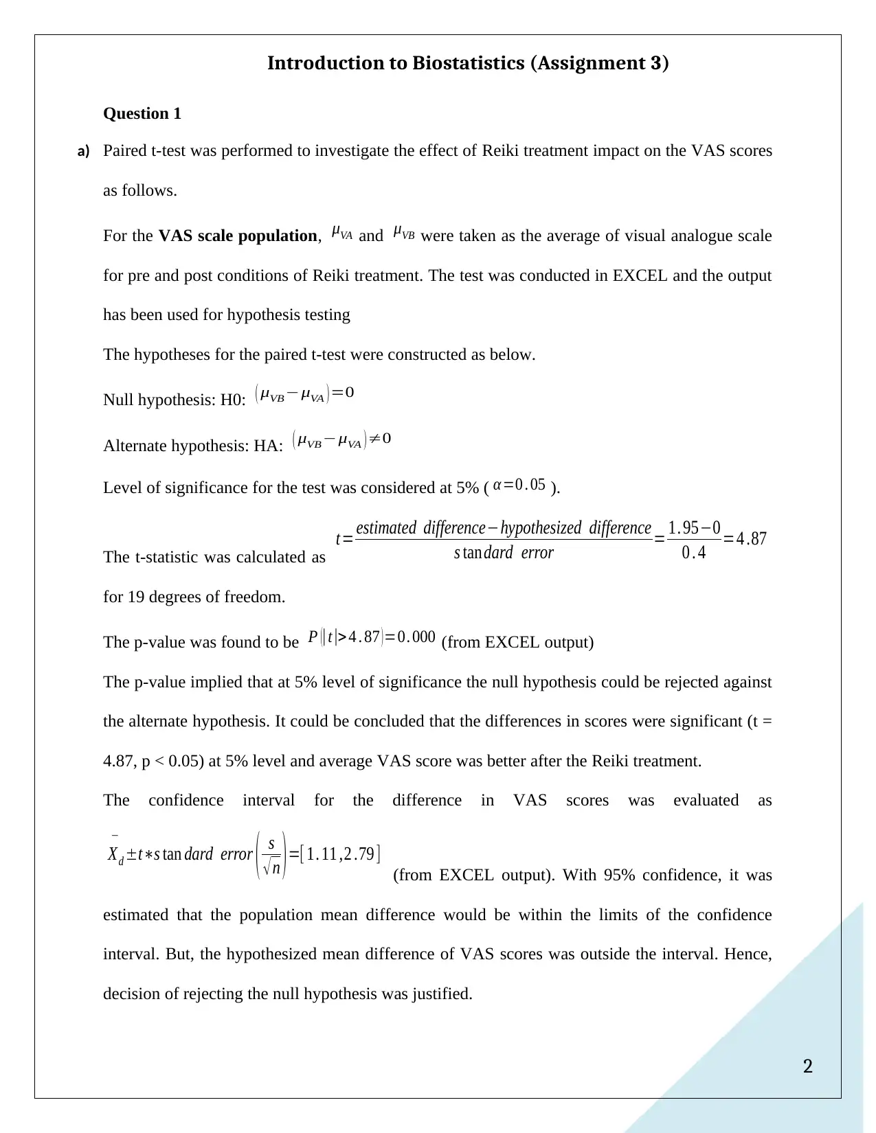
a) Paired t-test was performed to investigate the effect of Reiki treatment impact on the VAS scores
as follows.
For the VAS scale population, μVA and μVB were taken as the average of visual analogue scale
for pre and post conditions of Reiki treatment. The test was conducted in EXCEL and the output
has been used for hypothesis testing
The hypotheses for the paired t-test were constructed as below.
Null hypothesis: H0: ( μVB−μVA ) =0
Alternate hypothesis: HA: ( μVB−μVA ) ≠0
Level of significance for the test was considered at 5% ( α=0 . 05 ).
The t-statistic was calculated as
t= estimated difference−hypothesized difference
s tan dard error = 1. 95−0
0 . 4 =4 .87
for 19 degrees of freedom.
The p-value was found to be P (|t|> 4 . 87 ) =0. 000 (from EXCEL output)
The p-value implied that at 5% level of significance the null hypothesis could be rejected against
the alternate hypothesis. It could be concluded that the differences in scores were significant (t =
4.87, p < 0.05) at 5% level and average VAS score was better after the Reiki treatment.
The confidence interval for the difference in VAS scores was evaluated as
Xd
−
±t∗s tan dard error ( s
√ n ) =[ 1. 11 ,2 .79 ]
(from EXCEL output). With 95% confidence, it was
estimated that the population mean difference would be within the limits of the confidence
interval. But, the hypothesized mean difference of VAS scores was outside the interval. Hence,
decision of rejecting the null hypothesis was justified.
Introduction to Biostatistics (Assignment 3)
Question 1
a) Paired t-test was performed to investigate the effect of Reiki treatment impact on the VAS scores
as follows.
For the VAS scale population, μVA and μVB were taken as the average of visual analogue scale
for pre and post conditions of Reiki treatment. The test was conducted in EXCEL and the output
has been used for hypothesis testing
The hypotheses for the paired t-test were constructed as below.
Null hypothesis: H0: ( μVB−μVA ) =0
Alternate hypothesis: HA: ( μVB−μVA ) ≠0
Level of significance for the test was considered at 5% ( α=0 . 05 ).
The t-statistic was calculated as
t= estimated difference−hypothesized difference
s tan dard error = 1. 95−0
0 . 4 =4 .87
for 19 degrees of freedom.
The p-value was found to be P (|t|> 4 . 87 ) =0. 000 (from EXCEL output)
The p-value implied that at 5% level of significance the null hypothesis could be rejected against
the alternate hypothesis. It could be concluded that the differences in scores were significant (t =
4.87, p < 0.05) at 5% level and average VAS score was better after the Reiki treatment.
The confidence interval for the difference in VAS scores was evaluated as
Xd
−
±t∗s tan dard error ( s
√ n ) =[ 1. 11 ,2 .79 ]
(from EXCEL output). With 95% confidence, it was
estimated that the population mean difference would be within the limits of the confidence
interval. But, the hypothesized mean difference of VAS scores was outside the interval. Hence,
decision of rejecting the null hypothesis was justified.
3
Introduction to Biostatistics (Assignment 3)
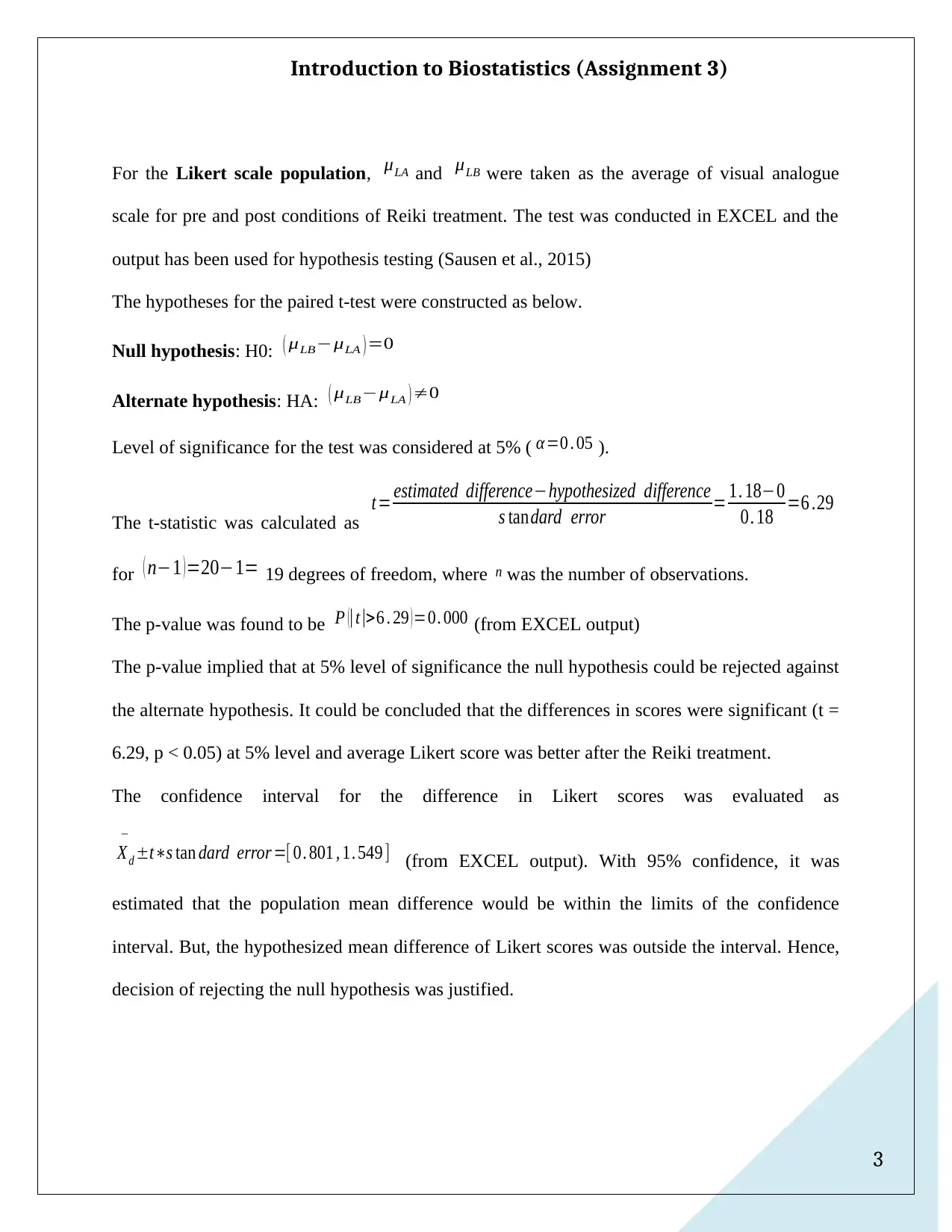
For the Likert scale population, μLA and μLB were taken as the average of visual analogue
scale for pre and post conditions of Reiki treatment. The test was conducted in EXCEL and the
output has been used for hypothesis testing (Sausen et al., 2015)
The hypotheses for the paired t-test were constructed as below.
Null hypothesis: H0: ( μLB−μLA ) =0
Alternate hypothesis: HA: ( μLB−μLA ) ≠0
Level of significance for the test was considered at 5% ( α=0 . 05 ).
The t-statistic was calculated as
t= estimated difference−hypothesized difference
s tan dard error = 1. 18−0
0. 18 =6 .29
for ( n−1 ) =20−1= 19 degrees of freedom, where n was the number of observations.
The p-value was found to be P (|t|>6 . 29 ) =0. 000 (from EXCEL output)
The p-value implied that at 5% level of significance the null hypothesis could be rejected against
the alternate hypothesis. It could be concluded that the differences in scores were significant (t =
6.29, p < 0.05) at 5% level and average Likert score was better after the Reiki treatment.
The confidence interval for the difference in Likert scores was evaluated as
Xd
−
±t∗s tan dard error =[ 0. 801 , 1. 549 ] (from EXCEL output). With 95% confidence, it was
estimated that the population mean difference would be within the limits of the confidence
interval. But, the hypothesized mean difference of Likert scores was outside the interval. Hence,
decision of rejecting the null hypothesis was justified.
Introduction to Biostatistics (Assignment 3)
For the Likert scale population, μLA and μLB were taken as the average of visual analogue
scale for pre and post conditions of Reiki treatment. The test was conducted in EXCEL and the
output has been used for hypothesis testing (Sausen et al., 2015)
The hypotheses for the paired t-test were constructed as below.
Null hypothesis: H0: ( μLB−μLA ) =0
Alternate hypothesis: HA: ( μLB−μLA ) ≠0
Level of significance for the test was considered at 5% ( α=0 . 05 ).
The t-statistic was calculated as
t= estimated difference−hypothesized difference
s tan dard error = 1. 18−0
0. 18 =6 .29
for ( n−1 ) =20−1= 19 degrees of freedom, where n was the number of observations.
The p-value was found to be P (|t|>6 . 29 ) =0. 000 (from EXCEL output)
The p-value implied that at 5% level of significance the null hypothesis could be rejected against
the alternate hypothesis. It could be concluded that the differences in scores were significant (t =
6.29, p < 0.05) at 5% level and average Likert score was better after the Reiki treatment.
The confidence interval for the difference in Likert scores was evaluated as
Xd
−
±t∗s tan dard error =[ 0. 801 , 1. 549 ] (from EXCEL output). With 95% confidence, it was
estimated that the population mean difference would be within the limits of the confidence
interval. But, the hypothesized mean difference of Likert scores was outside the interval. Hence,
decision of rejecting the null hypothesis was justified.
⊘ This is a preview!⊘
Do you want full access?
Subscribe today to unlock all pages.
Trusted by 1+ million students worldwide
4
Introduction to Biostatistics (Assignment 3)
Table 1: Paired t-test Output from EXCEL
Lower Upper
VAS before -
VAS after 1.95 1.79 0.40 1.11 2.79 4.87 19 0.000
Likert before -
Likert after 1.20 0.83 0.19 0.81 1.59 6.44 19 0.000
Paired t-test
Paired Differences
t df Sig. (2-tailed)
Mean Std. Deviation Std. Error Mean 95% Confidence
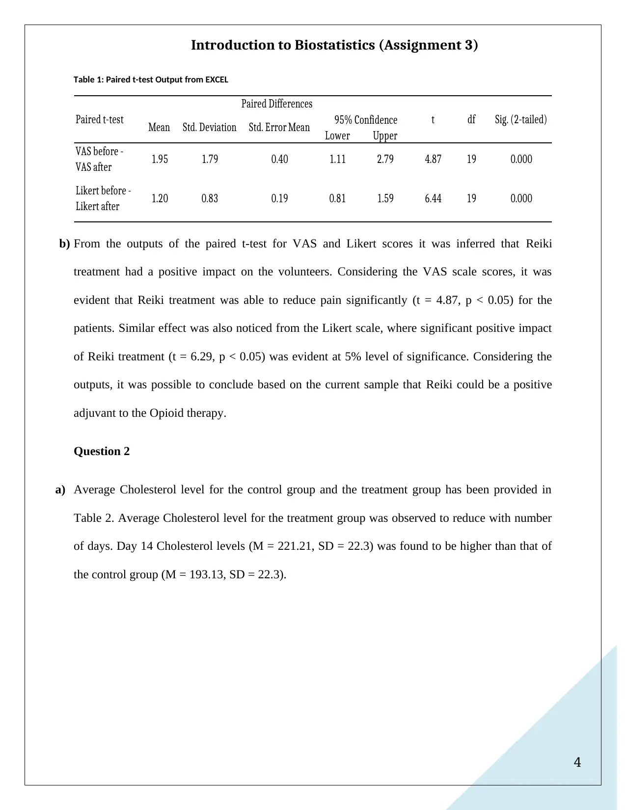
b) From the outputs of the paired t-test for VAS and Likert scores it was inferred that Reiki
treatment had a positive impact on the volunteers. Considering the VAS scale scores, it was
evident that Reiki treatment was able to reduce pain significantly (t = 4.87, p < 0.05) for the
patients. Similar effect was also noticed from the Likert scale, where significant positive impact
of Reiki treatment (t = 6.29, p < 0.05) was evident at 5% level of significance. Considering the
outputs, it was possible to conclude based on the current sample that Reiki could be a positive
adjuvant to the Opioid therapy.
Question 2
a) Average Cholesterol level for the control group and the treatment group has been provided in
Table 2. Average Cholesterol level for the treatment group was observed to reduce with number
of days. Day 14 Cholesterol levels (M = 221.21, SD = 22.3) was found to be higher than that of
the control group (M = 193.13, SD = 22.3).
Introduction to Biostatistics (Assignment 3)
Table 1: Paired t-test Output from EXCEL
Lower Upper
VAS before -
VAS after 1.95 1.79 0.40 1.11 2.79 4.87 19 0.000
Likert before -
Likert after 1.20 0.83 0.19 0.81 1.59 6.44 19 0.000
Paired t-test
Paired Differences
t df Sig. (2-tailed)
Mean Std. Deviation Std. Error Mean 95% Confidence
b) From the outputs of the paired t-test for VAS and Likert scores it was inferred that Reiki
treatment had a positive impact on the volunteers. Considering the VAS scale scores, it was
evident that Reiki treatment was able to reduce pain significantly (t = 4.87, p < 0.05) for the
patients. Similar effect was also noticed from the Likert scale, where significant positive impact
of Reiki treatment (t = 6.29, p < 0.05) was evident at 5% level of significance. Considering the
outputs, it was possible to conclude based on the current sample that Reiki could be a positive
adjuvant to the Opioid therapy.
Question 2
a) Average Cholesterol level for the control group and the treatment group has been provided in
Table 2. Average Cholesterol level for the treatment group was observed to reduce with number
of days. Day 14 Cholesterol levels (M = 221.21, SD = 22.3) was found to be higher than that of
the control group (M = 193.13, SD = 22.3).
Paraphrase This Document
Need a fresh take? Get an instant paraphrase of this document with our AI Paraphraser
5
Introduction to Biostatistics (Assignment 3)
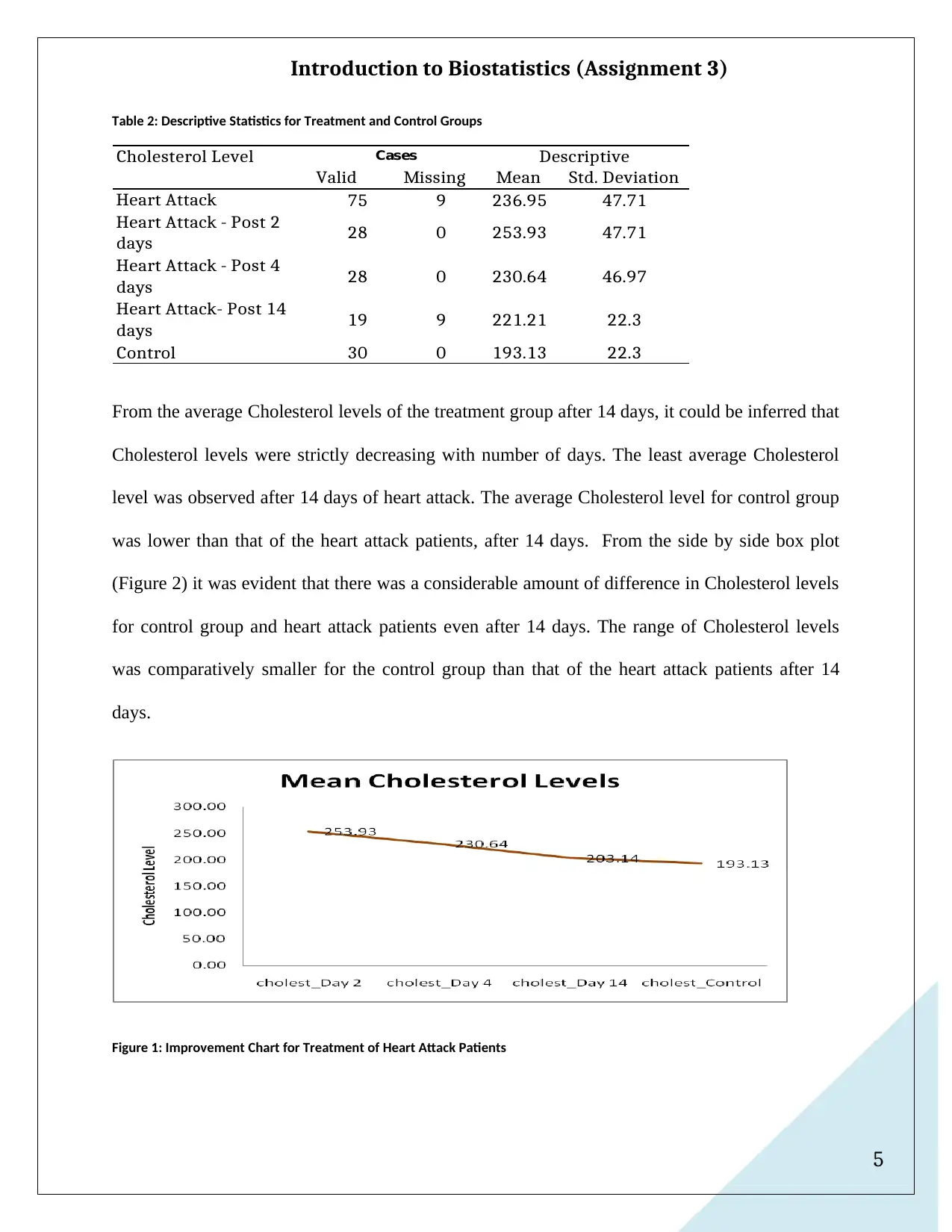
Table 2: Descriptive Statistics for Treatment and Control Groups
Valid Missing Mean Std. Deviation
Heart Attack 75 9 236.95 47.71
Heart Attack - Post 2
days 28 0 253.93 47.71
Heart Attack - Post 4
days 28 0 230.64 46.97
Heart Attack- Post 14
days 19 9 221.21 22.3
Control 30 0 193.13 22.3
Cholesterol Level Cases Descriptive
From the average Cholesterol levels of the treatment group after 14 days, it could be inferred that
Cholesterol levels were strictly decreasing with number of days. The least average Cholesterol
level was observed after 14 days of heart attack. The average Cholesterol level for control group
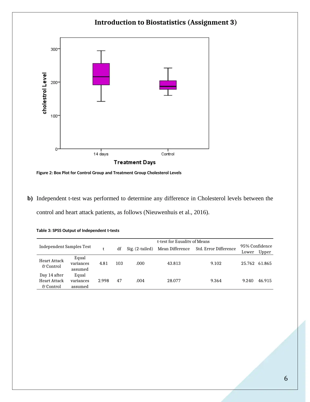
was lower than that of the heart attack patients, after 14 days. From the side by side box plot
(Figure 2) it was evident that there was a considerable amount of difference in Cholesterol levels
for control group and heart attack patients even after 14 days. The range of Cholesterol levels
was comparatively smaller for the control group than that of the heart attack patients after 14
days.
Figure 1: Improvement Chart for Treatment of Heart Attack Patients
Introduction to Biostatistics (Assignment 3)
Table 2: Descriptive Statistics for Treatment and Control Groups
Valid Missing Mean Std. Deviation
Heart Attack 75 9 236.95 47.71
Heart Attack - Post 2
days 28 0 253.93 47.71
Heart Attack - Post 4
days 28 0 230.64 46.97
Heart Attack- Post 14
days 19 9 221.21 22.3
Control 30 0 193.13 22.3
Cholesterol Level Cases Descriptive
From the average Cholesterol levels of the treatment group after 14 days, it could be inferred that
Cholesterol levels were strictly decreasing with number of days. The least average Cholesterol
level was observed after 14 days of heart attack. The average Cholesterol level for control group
was lower than that of the heart attack patients, after 14 days. From the side by side box plot
(Figure 2) it was evident that there was a considerable amount of difference in Cholesterol levels
for control group and heart attack patients even after 14 days. The range of Cholesterol levels
was comparatively smaller for the control group than that of the heart attack patients after 14
days.
Figure 1: Improvement Chart for Treatment of Heart Attack Patients
6
Introduction to Biostatistics (Assignment 3)
Figure 2: Box Plot for Control Group and Treatment Group Cholesterol Levels
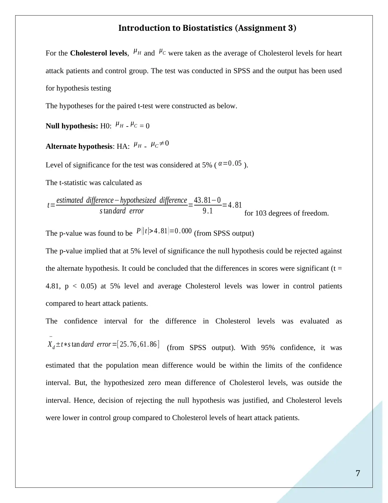
b) Independent t-test was performed to determine any difference in Cholesterol levels between the
control and heart attack patients, as follows (Nieuwenhuis et al., 2016).
Table 3: SPSS Output of Independent t-tests
Lower Upper
Heart Attack
& Control
Equal
variances
assumed
4.81 103 .000 43.813 9.102 25.762 61.865
Day 14 after
Heart Attack
& Control
Equal
variances
assumed
2.998 47 .004 28.077 9.364 9.240 46.915
Std. Error Difference 95% ConfidenceIndependent Samples Test
t-test for Equality of Means
t df Sig. (2-tailed) Mean Difference
Introduction to Biostatistics (Assignment 3)
Figure 2: Box Plot for Control Group and Treatment Group Cholesterol Levels
b) Independent t-test was performed to determine any difference in Cholesterol levels between the
control and heart attack patients, as follows (Nieuwenhuis et al., 2016).
Table 3: SPSS Output of Independent t-tests
Lower Upper
Heart Attack
& Control
Equal
variances
assumed
4.81 103 .000 43.813 9.102 25.762 61.865
Day 14 after
Heart Attack
& Control
Equal
variances
assumed
2.998 47 .004 28.077 9.364 9.240 46.915
Std. Error Difference 95% ConfidenceIndependent Samples Test
t-test for Equality of Means
t df Sig. (2-tailed) Mean Difference
⊘ This is a preview!⊘
Do you want full access?
Subscribe today to unlock all pages.
Trusted by 1+ million students worldwide
7
Introduction to Biostatistics (Assignment 3)
For the Cholesterol levels, μH and μC were taken as the average of Cholesterol levels for heart
attack patients and control group. The test was conducted in SPSS and the output has been used
for hypothesis testing
The hypotheses for the paired t-test were constructed as below.
Null hypothesis: H0: μH - μC = 0
Alternate hypothesis: HA: μH - μC≠0
Level of significance for the test was considered at 5% ( α=0 . 05 ).
The t-statistic was calculated as
t= estimated difference−hypothesized difference
s tandard error =43. 81−0
9 .1 =4 . 81 for 103 degrees of freedom.
The p-value was found to be P (|t|> 4 . 81 ) =0 . 000 (from SPSS output)
The p-value implied that at 5% level of significance the null hypothesis could be rejected against
the alternate hypothesis. It could be concluded that the differences in scores were significant (t =
4.81, p < 0.05) at 5% level and average Cholesterol levels was lower in control patients
compared to heart attack patients.
The confidence interval for the difference in Cholesterol levels was evaluated as
Xd
−
±t∗s tan dard error =[ 25. 76 , 61. 86 ] (from SPSS output). With 95% confidence, it was
estimated that the population mean difference would be within the limits of the confidence
interval. But, the hypothesized zero mean difference of Cholesterol levels, was outside the
interval. Hence, decision of rejecting the null hypothesis was justified, and Cholesterol levels
were lower in control group compared to Cholesterol levels of heart attack patients.
Paraphrase This Document
Need a fresh take? Get an instant paraphrase of this document with our AI Paraphraser
8
Introduction to Biostatistics (Assignment 3)
Now, especially for the Cholesterol levels in heart attack patients after 14 days, μ14 and μC
were taken as the average of Cholesterol levels for heart attack patients and control group. The
test was conducted in SPSS and the output has been used for hypothesis testing
The hypotheses for the paired t-test were constructed as below.
Null hypothesis: H0: μ14 - μC = 0
Alternate hypothesis: HA: μ14 - μC≠0
Level of significance for the test was considered at 5% ( α=0 . 05 ).
The t-statistic was calculated as
t= estimated difference−hypothesized difference
s tandard error =28 . 07−0
9 .36 =2 . 998 for 103 degrees of freedom.
The p-value was found to be P (|t|>2 . 998 ) =0 . 004 (from SPSS output)
The p-value implied that at 5% level of significance the null hypothesis could be rejected against
the alternate hypothesis. It could be concluded that the differences in scores were significant (t =
2.99, p < 0.05) at 5% level and average Cholesterol levels was lower in control patients
compared to heart attack patients after 14 days.
The confidence interval for the difference in Cholesterol levels was evaluated as
Xd
−
±t∗s tan dard error =[ 9 .24 , 46 .91 ] (from SPSS output). With 95% confidence, it was estimated
that the population mean difference would be within the limits of the confidence interval. But,
the hypothesized zero mean difference of Cholesterol levels, was outside the interval. Hence,
decision of rejecting the null hypothesis was justified, and Cholesterol levels were lower in
control group compared to Cholesterol levels of heart attack patients after 14 days
9
Introduction to Biostatistics (Assignment 3)
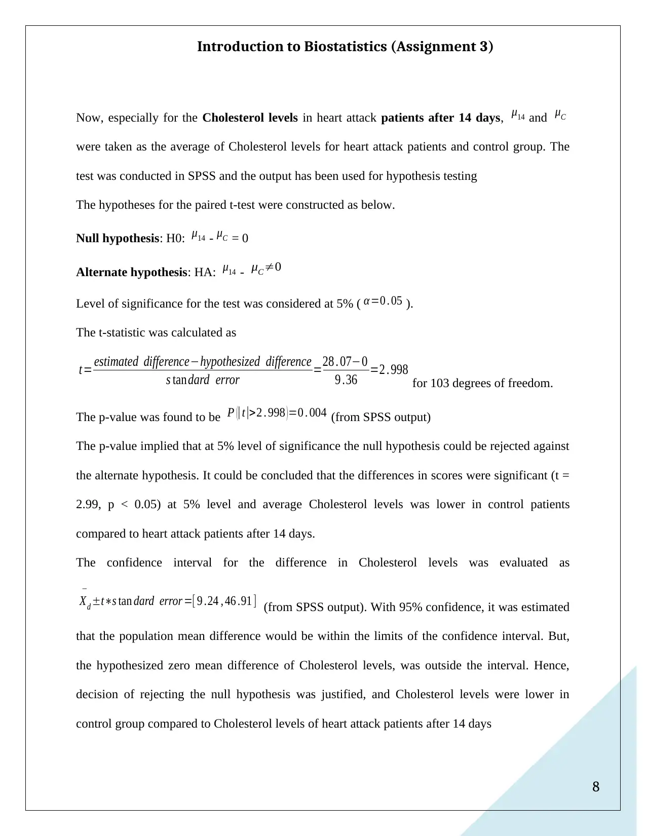
c) The population parameters were not available to evaluate the value of the test statistic. Hence,
choice of Student’s t-test was obvious rather than the Z-test statistic. But, the normality
assumption of the independent t-test for the present data was not satisfied. For the Cholesterol
levels of the volunteers. From Shapiro Wilk test it was found (SW = 0.98, p = 0.2) that the null
hypothesis could not get rejected, and the Cholesterol levels was not normal. Hence, a non
parametric test (Mann- Whitney U – test) would have been a better choice (MacFarland, and
Yates, 2016).
Figure 3: Cholesterol Level of Heart Attack patients (Negative Skewed)
Introduction to Biostatistics (Assignment 3)
c) The population parameters were not available to evaluate the value of the test statistic. Hence,
choice of Student’s t-test was obvious rather than the Z-test statistic. But, the normality
assumption of the independent t-test for the present data was not satisfied. For the Cholesterol
levels of the volunteers. From Shapiro Wilk test it was found (SW = 0.98, p = 0.2) that the null
hypothesis could not get rejected, and the Cholesterol levels was not normal. Hence, a non
parametric test (Mann- Whitney U – test) would have been a better choice (MacFarland, and
Yates, 2016).
Figure 3: Cholesterol Level of Heart Attack patients (Negative Skewed)
⊘ This is a preview!⊘
Do you want full access?
Subscribe today to unlock all pages.
Trusted by 1+ million students worldwide
10
Introduction to Biostatistics (Assignment 3)
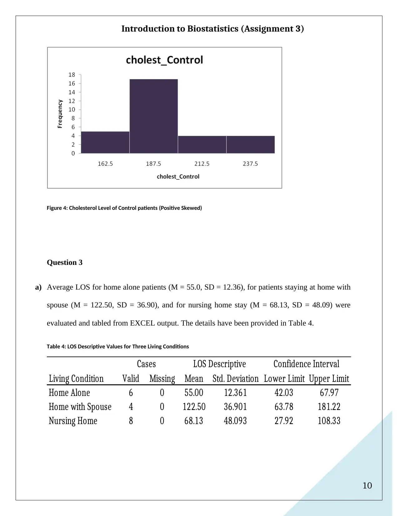
Figure 4: Cholesterol Level of Control patients (Positive Skewed)
Question 3
a) Average LOS for home alone patients (M = 55.0, SD = 12.36), for patients staying at home with
spouse (M = 122.50, SD = 36.90), and for nursing home stay (M = 68.13, SD = 48.09) were
evaluated and tabled from EXCEL output. The details have been provided in Table 4.
Table 4: LOS Descriptive Values for Three Living Conditions
Living Condition Valid Missing Mean Std. Deviation Lower Limit Upper Limit
Home Alone 6 0 55.00 12.361 42.03 67.97
Home with Spouse 4 0 122.50 36.901 63.78 181.22
Nursing Home 8 0 68.13 48.093 27.92 108.33
Cases LOS Descriptive Confidence Interval
Introduction to Biostatistics (Assignment 3)
Figure 4: Cholesterol Level of Control patients (Positive Skewed)
Question 3
a) Average LOS for home alone patients (M = 55.0, SD = 12.36), for patients staying at home with
spouse (M = 122.50, SD = 36.90), and for nursing home stay (M = 68.13, SD = 48.09) were
evaluated and tabled from EXCEL output. The details have been provided in Table 4.
Table 4: LOS Descriptive Values for Three Living Conditions
Living Condition Valid Missing Mean Std. Deviation Lower Limit Upper Limit
Home Alone 6 0 55.00 12.361 42.03 67.97
Home with Spouse 4 0 122.50 36.901 63.78 181.22
Nursing Home 8 0 68.13 48.093 27.92 108.33
Cases LOS Descriptive Confidence Interval
Paraphrase This Document
Need a fresh take? Get an instant paraphrase of this document with our AI Paraphraser
11
Introduction to Biostatistics (Assignment 3)
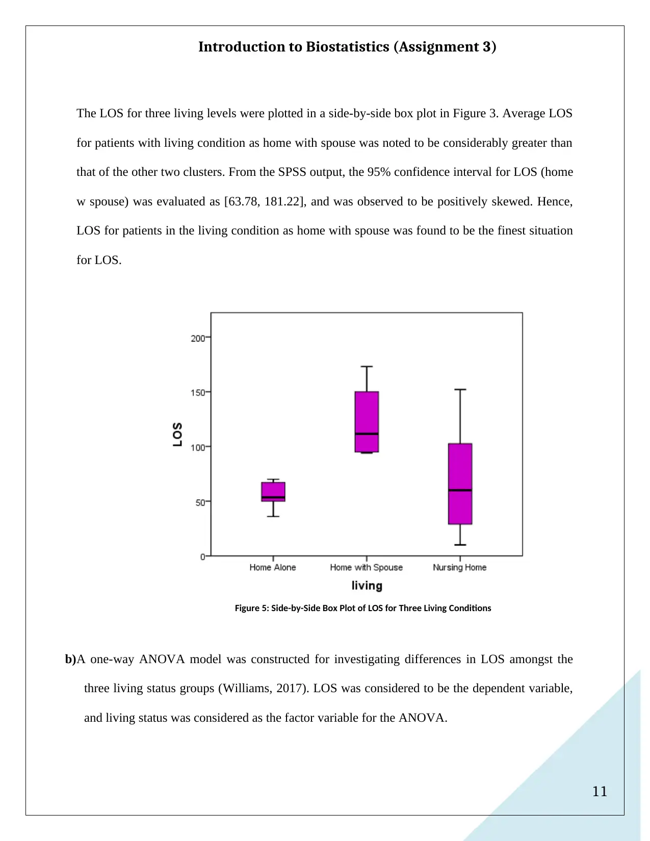
The LOS for three living levels were plotted in a side-by-side box plot in Figure 3. Average LOS
for patients with living condition as home with spouse was noted to be considerably greater than
that of the other two clusters. From the SPSS output, the 95% confidence interval for LOS (home
w spouse) was evaluated as [63.78, 181.22], and was observed to be positively skewed. Hence,
LOS for patients in the living condition as home with spouse was found to be the finest situation
for LOS.
Figure 5: Side-by-Side Box Plot of LOS for Three Living Conditions
b)A one-way ANOVA model was constructed for investigating differences in LOS amongst the
three living status groups (Williams, 2017). LOS was considered to be the dependent variable,
and living status was considered as the factor variable for the ANOVA.
Introduction to Biostatistics (Assignment 3)
The LOS for three living levels were plotted in a side-by-side box plot in Figure 3. Average LOS
for patients with living condition as home with spouse was noted to be considerably greater than
that of the other two clusters. From the SPSS output, the 95% confidence interval for LOS (home
w spouse) was evaluated as [63.78, 181.22], and was observed to be positively skewed. Hence,
LOS for patients in the living condition as home with spouse was found to be the finest situation
for LOS.
Figure 5: Side-by-Side Box Plot of LOS for Three Living Conditions
b)A one-way ANOVA model was constructed for investigating differences in LOS amongst the
three living status groups (Williams, 2017). LOS was considered to be the dependent variable,
and living status was considered as the factor variable for the ANOVA.
12
Introduction to Biostatistics (Assignment 3)
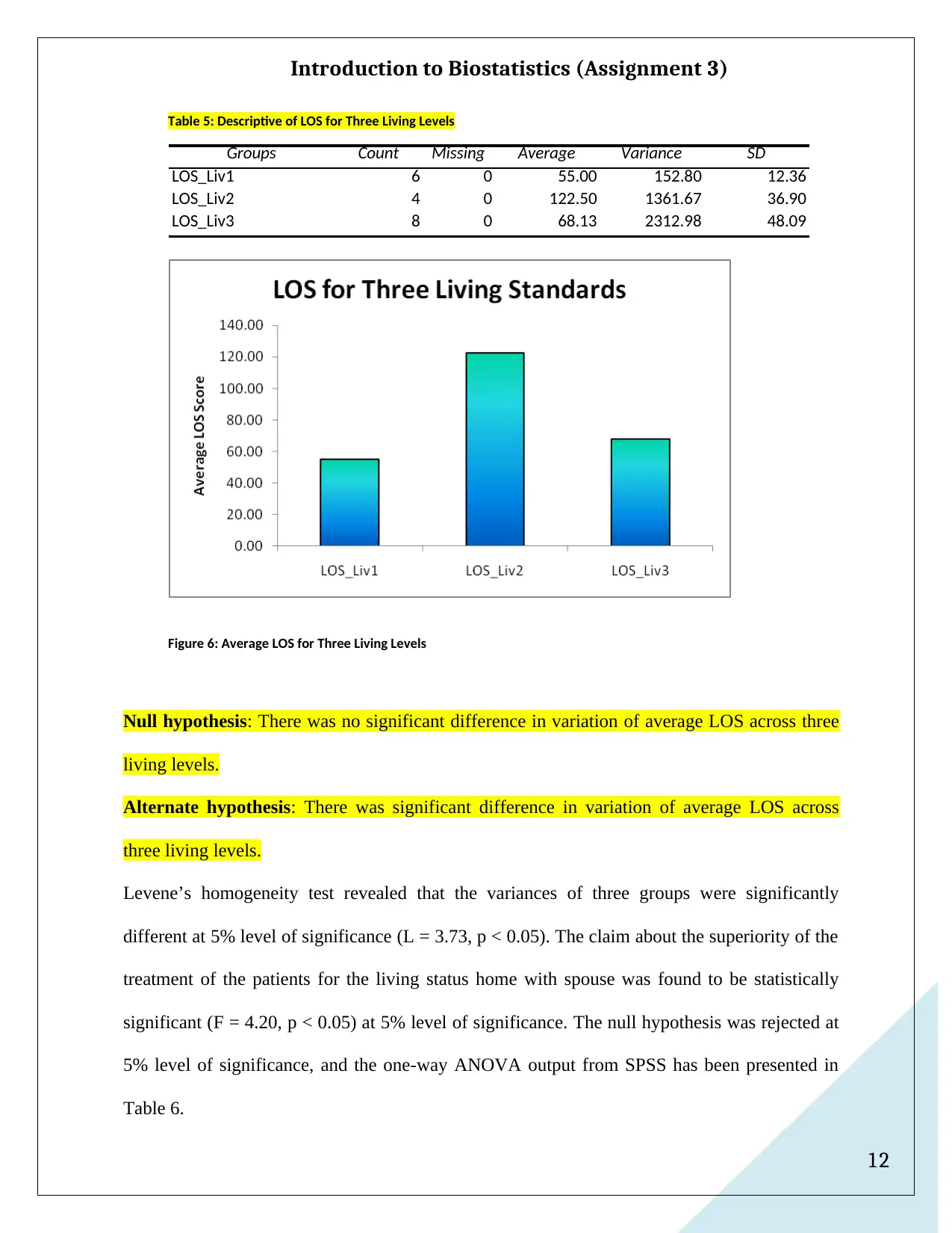
Table 5: Descriptive of LOS for Three Living Levels
Groups Count Missing Average Variance SD
LOS_Liv1 6 0 55.00 152.80 12.36
LOS_Liv2 4 0 122.50 1361.67 36.90
LOS_Liv3 8 0 68.13 2312.98 48.09
Figure 6: Average LOS for Three Living Levels
Null hypothesis: There was no significant difference in variation of average LOS across three
living levels.
Alternate hypothesis: There was significant difference in variation of average LOS across
three living levels.
Levene’s homogeneity test revealed that the variances of three groups were significantly
different at 5% level of significance (L = 3.73, p < 0.05). The claim about the superiority of the
treatment of the patients for the living status home with spouse was found to be statistically
significant (F = 4.20, p < 0.05) at 5% level of significance. The null hypothesis was rejected at
5% level of significance, and the one-way ANOVA output from SPSS has been presented in
Table 6.
Introduction to Biostatistics (Assignment 3)
Table 5: Descriptive of LOS for Three Living Levels
Groups Count Missing Average Variance SD
LOS_Liv1 6 0 55.00 152.80 12.36
LOS_Liv2 4 0 122.50 1361.67 36.90
LOS_Liv3 8 0 68.13 2312.98 48.09
Figure 6: Average LOS for Three Living Levels
Null hypothesis: There was no significant difference in variation of average LOS across three
living levels.
Alternate hypothesis: There was significant difference in variation of average LOS across
three living levels.
Levene’s homogeneity test revealed that the variances of three groups were significantly
different at 5% level of significance (L = 3.73, p < 0.05). The claim about the superiority of the
treatment of the patients for the living status home with spouse was found to be statistically
significant (F = 4.20, p < 0.05) at 5% level of significance. The null hypothesis was rejected at
5% level of significance, and the one-way ANOVA output from SPSS has been presented in
Table 6.
⊘ This is a preview!⊘
Do you want full access?
Subscribe today to unlock all pages.
Trusted by 1+ million students worldwide
1 out of 18
Related Documents


Your All-in-One AI-Powered Toolkit for Academic Success.
+13062052269
info@desklib.com
Available 24*7 on WhatsApp / Email
![[object Object]](/_next/static/media/star-bottom.7253800d.svg)
Unlock your academic potential
Copyright © 2020–2026 A2Z Services. All Rights Reserved. Developed and managed by ZUCOL.