Biostatistics: STROBE Checklist Application and Work Hours Analysis

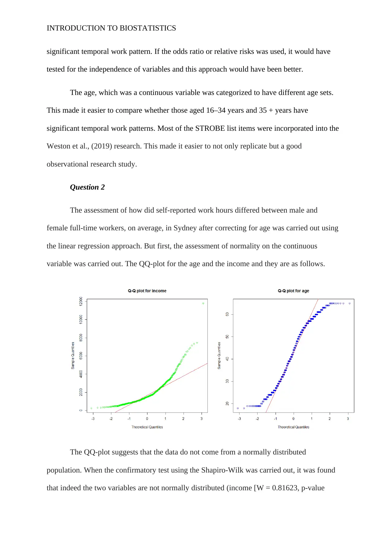
This assignment critically appraises a research paper using the STROBE checklist, focusing on items related to statistical methods and reporting. It evaluates how the study addresses sample selection, statistical analyses, and participant characteristics. Additionally, the assignment includes a linear regression analysis to assess the relationship between self-reported work hours, age, and gender among full-time workers in Sydney, examining normality, model significance, and coefficient interpretation to predict work hours based on gender and age. The report also highlights the limitations based on the coefficient of determination.

Running head: INTRODUCTION TO BIOSTATISTICS
Introduction to Biostatistics
Name:
Institution:

INTRODUCTION TO BIOSTATISTICS
Question 1
The STROBE item number ten, which addresses how the sample was obtained was
addressed briefly. The research used a second phase sample data from the UK Household
Longitudinal Study (UKHLS) (Weston, Zilanawala, Webb, Carvalho, & McMunn, 2019).
The second phase data was used simply because main variable of interest “weekends
working” and “work conditions” were included. All the people in the data were used as the
sample (a total of 11215 men and 12188). The flow diagram for the data selection was not
used, but the description given was clear enough to understand why the selected data were
used. Item twelve in the STROBE checklist is partially met. First, the statistical methods used
to find answers the primary objective were highlighted. The inclusion of statistical analysis
was crucial as it makes it possible for the replication of similar research. The missing data
were imputed using the multiple imputations by chained equations. In the report formal test
for the interaction effect for gender was not shown, the researcher indicated that they were
available on request. Also, the research did not cover any sensitivity analysis.
The potential individuals eligible in the data were identified, and those with preferred
variables included in the study. Thus, STROBE item thirteen was achieved. The researcher
identified the characteristics of the study participants. In addition, the covariates that were
adjusted were highlighted. For instance, the researcher indicated that age and age squared,
education attainment, marital status, among other factors were adjusted for. The main reason
for adjustments was given; like the case of age and age squared, it was adjusted because
trajectories indicated that depressive symptoms in adulthood have a u-shaped. Thus, the
adjustments were deemed necessary. This made it easier to account for their effect and make
the association somehow linear. The relative risks and odds ratios were not reported rather
unadjusted mean confidence interval was used to determine whether men and women had a

INTRODUCTION TO BIOSTATISTICS
significant temporal work pattern. If the odds ratio or relative risks was used, it would have
tested for the independence of variables and this approach would have been better.
The age, which was a continuous variable was categorized to have different age sets.
This made it easier to compare whether those aged 16–34 years and 35 + years have
significant temporal work patterns. Most of the STROBE list items were incorporated into the
Weston et al., (2019) research. This made it easier to not only replicate but a good
observational research study.
Question 2
The assessment of how did self-reported work hours differed between male and
female full-time workers, on average, in Sydney after correcting for age was carried out using
the linear regression approach. But first, the assessment of normality on the continuous
variable was carried out. The QQ-plot for the age and the income and they are as follows.
The QQ-plot suggests that the data do not come from a normally distributed
population. When the confirmatory test using the Shapiro-Wilk was carried out, it was found
that indeed the two variables are not normally distributed (income [W = 0.81623, p-value

INTRODUCTION TO BIOSTATISTICS
< .05] and age [W = 0.94941, p-value <.05]) (Cohen, West, & Aiken, 2014). We fit a
multiple linear regression on the data to test the hypothesis: H0: there is a linear relationship
between the self-reported work hours and the age of the workers and gender. The analysis
was carried out at the level .05. Thus, we should reject the null hypothesis if the p-value is
less than the level α = .05.
The fitted linear regression model is as follows:
Work = 42.76497 - 0.01956(age) -5.55532 (sex)
In this case, the female is the baseline of contrast. The model in this case, is
significant (F (2, 495) = 68.65, p-value < .05) (Cohen, West, & Aiken, 2014). This model can
be used to make predictions since it is significant. However, when the coefficients were
tested whether they were significant, only the sex coefficient was significant (t (495) = -
11.687, p-value < .05). The coefficient of determination indicates that the fitted model can
explain 21.71% of sources of variation. This proportion of variation is quite low to ascertain
the validity of the model. However, we can still use the model to make predictions. We
consider a case, where an individual is a male aged 25 years, and make the prediction of the
hours worked.
Work = 42.76497 - 0.01956(25) -5.55532 (0); male = 0
= 42.27597
The prediction for a female aged 25 years is as follows.
Work = 42.76497 - 0.01956(25) -5.55532 (1); female = 1
= 36.72065
The summary indicates that female workers are expected to work for fewer hours than
male workers. In this model, the age coefficient is negative, which suggests that as people get

INTRODUCTION TO BIOSTATISTICS
old, they are expected to work for fewer hours. In other words, old people are expected to
work for fewer hours. The coefficient for gender indicates that on average female works
5.55532 hours less than the male workers. Based, on the model results this average difference
is statistically different.

INTRODUCTION TO BIOSTATISTICS
References
Cohen, P., West, S. G., & Aiken, L. S. (2014). Applied multiple regression/correlation
analysis for the behavioral sciences (2nd ed.). Psychology Press.
Weston, G., Zilanawala, A., Webb, E., Carvalho, L. A., & McMunn, A. (2019). Weston, G.,
Zilanawala, A., Webb, E., Carvalho, L. A., & McMunn, A. (2019). Long work hours,
weekend working and depressive symptoms in men and women: findings from a UK
population-based study. J Epidemiol Community Health, 1-10.