Statistical Analysis of Weight, Exercise, and Gender Data - 2017

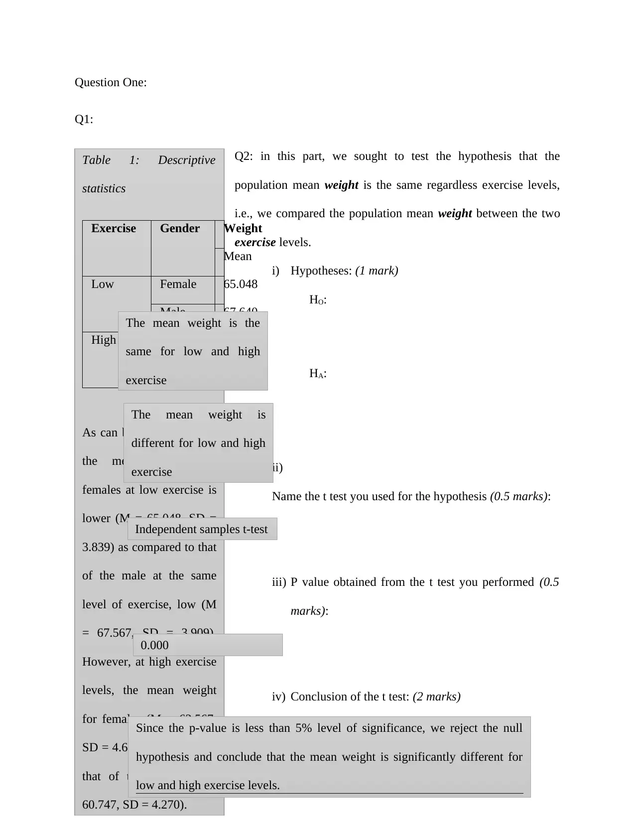
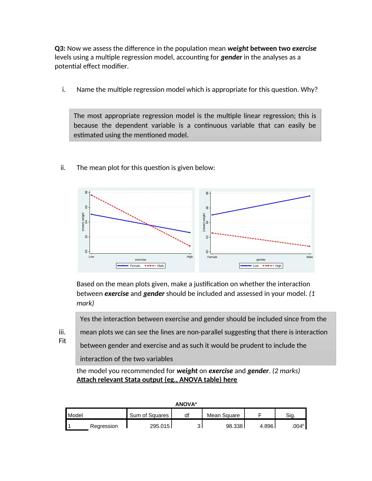
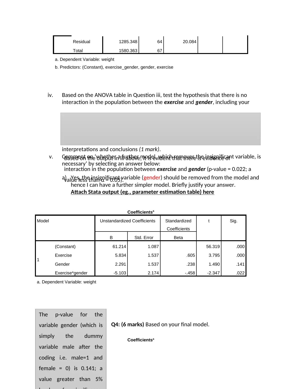
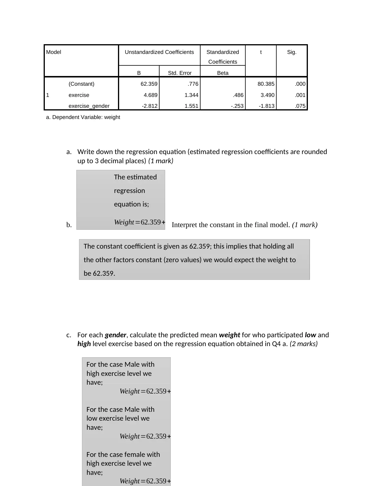
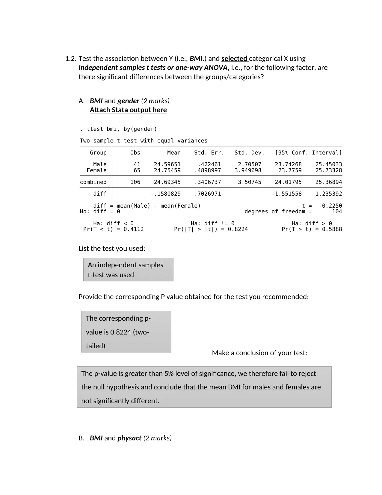
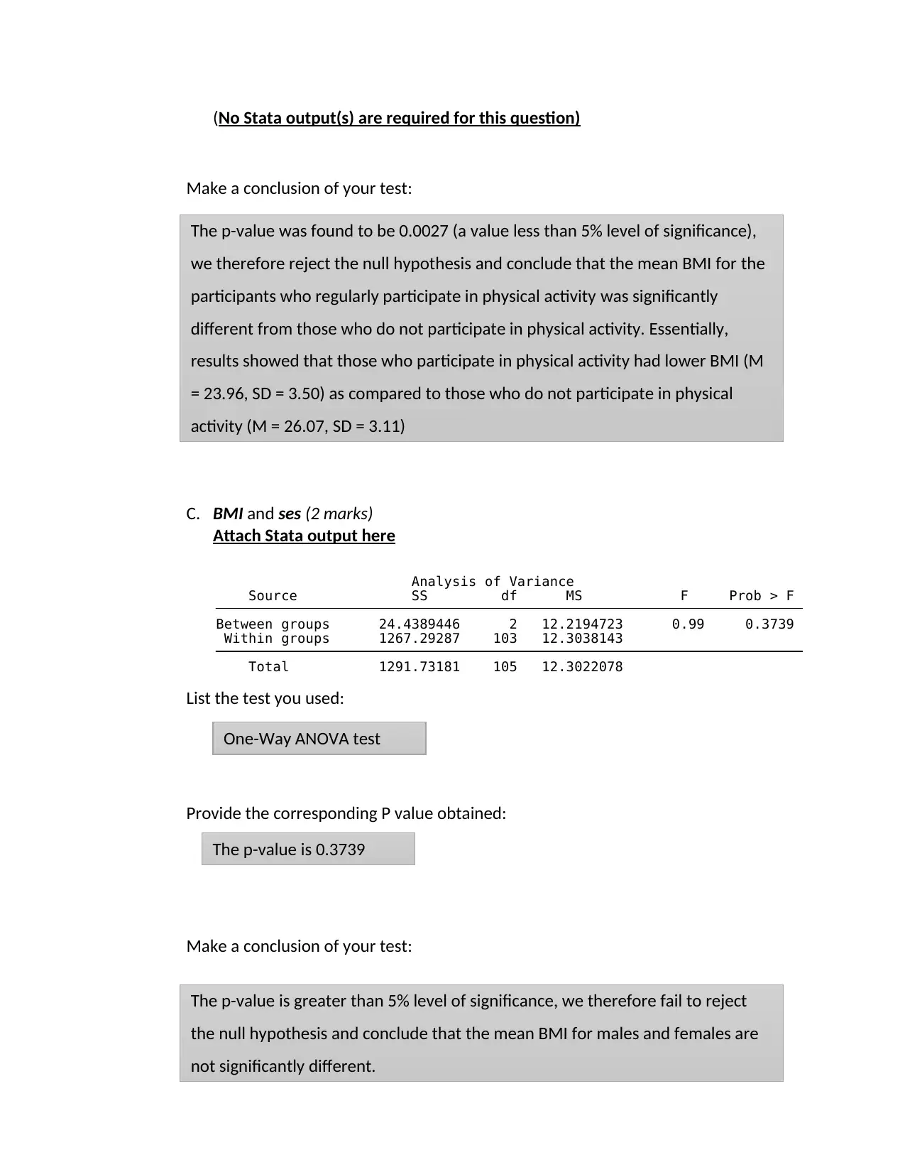
This biostatistics assignment presents a comprehensive analysis of weight data, exploring the relationships between weight, exercise levels, and gender. The assignment begins with descriptive statistics, comparing the mean weights of males and females at low and high exercise levels. It then tests the hypothesis that population mean weight is the same regardless of exercise levels using an independent samples t-test, followed by a multiple regression model to assess the influence of exercise and gender on weight, including interaction effects. The student justifies the inclusion of an interaction term based on mean plots and tests for its significance using ANOVA. Furthermore, the assignment involves model interpretation, including the regression equation and interpretation of coefficients, and calculations of predicted mean weights for different gender and exercise level combinations. Finally, the assignment investigates the relationship between BMI and age using correlation, and the association between BMI and categorical variables like gender, physical activity, and socioeconomic status using t-tests and ANOVA, providing conclusions based on statistical outputs.

Epidemiology and Biostatistics
Name
Student’s Number
Professor’s Name
6th October 2017

Question One:
Q1:
Q2: in this part, we sought to test the hypothesis that the
population mean weight is the same regardless exercise levels,
i.e., we compared the population mean weight between the two
exercise levels.
i) Hypotheses: (1 mark)
HO:
HA:
ii)
Name the t test you used for the hypothesis (0.5 marks):
iii) P value obtained from the t test you performed (0.5
marks):
iv) Conclusion of the t test: (2 marks)
Table 1: Descriptive
statistics
Exercise Gender Weight
Mean
Low Female 65.048
Male 67.640
High Female 62.567
Male 60.747
As can be seen in table 1,
the mean weight for
females at low exercise is
lower (M = 65.048, SD =
3.839) as compared to that
of the male at the same
level of exercise, low (M
= 67.567, SD = 3.909).
However, at high exercise
levels, the mean weight
for females (M = 62.567,
SD = 4.673) is higher than
that of the males (M =
60.747, SD = 4.270).
The mean weight is the
same for low and high
exercise
The mean weight is
different for low and high
exercise
Independent samples t-test
0.000
Since the p-value is less than 5% level of significance, we reject the null
hypothesis and conclude that the mean weight is significantly different for
low and high exercise levels.

Q3: Now we assess the difference in the population mean weight between two exercise
levels using a multiple regression model, accounting for gender in the analyses as a
potential effect modifier.
i. Name the multiple regression model which is appropriate for this question. Why?
ii. The mean plot for this question is given below:
60 62 64 66 68
(mean) weight
Low High
exercise
Female Male
60 62 64 66 68
(mean) weight
MaleFemale gender
Low High
Based on the mean plots given, make a justification on whether the interaction
between exercise and gender should be included and assessed in your model. (1
mark)
iii.
Fit
the model you recommended for weight on exercise and gender. (2 marks)
Attach relevant Stata output (eg., ANOVA table) here
ANOVAa
Model Sum of Squares df Mean Square F Sig.
1 Regression 295.015 3 98.338 4.896 .004b
The most appropriate regression model is the multiple linear regression; this is
because the dependent variable is a continuous variable that can easily be
estimated using the mentioned model.
Yes the interaction between exercise and gender should be included since from the
mean plots we can see the lines are non-parallel suggesting that there is interaction
between gender and exercise and as such it would be prudent to include the
interaction of the two variables

Residual 1285.348 64 20.084
Total 1580.363 67
a. Dependent Variable: weight
b. Predictors: (Constant), exercise_gender, gender, exercise
iv. Based on the ANOVA table in Question iii, test the hypothesis that there is no
interaction in the population between the exercise and gender, including your
interpretations and conclusions (1 mark).
v. Comment on ‘whether a further model, which removes the insignificant variable, is
necessary’ by selecting an answer below:
a) Yes, the insignificant variable (gender) should be removed from the model and
hence I can have a further simpler model. Briefly justify your answer.
Attach Stata output (eg., parameter estimation table) here
Coefficientsa
Model Unstandardized Coefficients Standardized
Coefficients
t Sig.
B Std. Error Beta
1
(Constant) 61.214 1.087 56.319 .000
Exercise 5.834 1.537 .605 3.795 .000
Gender 2.291 1.537 .238 1.490 .141
Exercise*gender -5.103 2.174 -.458 -2.347 .022
a. Dependent Variable: weight
Q4: (6 marks) Based on your final model.
Coefficientsa
Based on the output in iii above, it is evident that there is evidence of
interaction in the population between exercise and gender (p-value = 0.022; a
value less than α = 0.05).
The p-value for the
variable gender (which is
simply the dummy
variable male after the
coding i.e. male=1 and
female = 0) is 0.141; a
value greater than 5%

Model Unstandardized Coefficients Standardized
Coefficients
t Sig.
B Std. Error Beta
1
(Constant) 62.359 .776 80.385 .000
exercise 4.689 1.344 .486 3.490 .001
exercise_gender -2.812 1.551 -.253 -1.813 .075
a. Dependent Variable: weight
a. Write down the regression equation (estimated regression coefficients are rounded
up to 3 decimal places) (1 mark)
b. Interpret the constant in the final model. (1 mark)
c. For each gender, calculate the predicted mean weight for who participated low and
high level exercise based on the regression equation obtained in Q4 a. (2 marks)
The estimated
regression
equation is;
Weight=62.359+4.689 ( High ) −2.812(HighMale)
The constant coefficient is given as 62.359; this implies that holding all
the other factors constant (zero values) we would expect the weight to
be 62.359.
For the case Male with
high exercise level we
have;
Weight=62.359+ 4.689 ( 1 )−2.812 ( 1 )=64.236
For the case Male with
low exercise level we
have;
Weight=62.359+4.689 ( 0 ) −2.812 ( 0 ) =62.359
For the case female with
high exercise level we
have;
Weight=62.359+4.689 ( 1 ) −2.812 ( 0 ) =67.048

d. Do you agree that the regression coefficient n‘6.894’ could be interpreted as
‘Subjects who participated in low level exercises were heavier by 6.894 kg on
average than those who participated in high level exercises regardless gender’? (2
marks)
2. (4 marks) Using information you obtained in Q4, make a detailed conclusion with regard to
the research aim.
QUESTION TWO
1. (7 marks) Exploratory analyses using descriptive statistics and plots.
1.1. Examine the linear relationship between BMI and age using scatter plot and
Pearson’s correlation coefficient. What is your conclusion? (1 mark)
(No Stata output(s) are required for this question)
The Pearson correlation coefficient between age and BMI was found to be
0.2615; this implies a weak positive relationship between the two variables (Age
and BMI). The correlation was however found to be significant at 5% significance
level (p-value < 0.05).
For the case female with
Yes. I agree because exercise is a categorical variable that when
coded 1 for low exercise would be compared with the high
levels.
The aim of the research was to find out the relationship that exists between an
individual’s weight and two factors which are gender of the individual and the
individual’s level of physical exercise. Results showed that there was no
significant relationship between gender and weight however there was significant
relationship between exercise and weight and also between interaction between
exercise and gender and weight of an individual.
Final regression equation showed that if all the factors are held constant, the
weight of individuals in the sample would be 62.359.

1.2. Test the association between Y (i.e., BMI.) and selected categorical X using
independent samples t tests or one-way ANOVA, i.e., for the following factor, are
there significant differences between the groups/categories?
A. BMI and gender (2 marks)
Attach Stata output here
Pr(T < t) = 0.4112 Pr(|T| > |t|) = 0.8224 Pr(T > t) = 0.5888
Ha: diff < 0 Ha: diff != 0 Ha: diff > 0
Ho: diff = 0 degrees of freedom = 104
diff = mean(Male) - mean(Female) t = -0.2250
diff -.1580829 .7026971 -1.551558 1.235392
combined 106 24.69345 .3406737 3.50745 24.01795 25.36894
Female 65 24.75459 .4898997 3.949698 23.7759 25.73328
Male 41 24.59651 .422461 2.70507 23.74268 25.45033
Group Obs Mean Std. Err. Std. Dev. [95% Conf. Interval]
Two-sample t test with equal variances
. ttest bmi, by(gender)
List the test you used:
Provide the corresponding P value obtained for the test you recommended:
Make a conclusion of your test:
B. BMI and physact (2 marks)
An independent samples
t-test was used
The corresponding p-
value is 0.8224 (two-
tailed)
The p-value is greater than 5% level of significance, we therefore fail to reject
the null hypothesis and conclude that the mean BMI for males and females are
not significantly different.

(No Stata output(s) are required for this question)
Make a conclusion of your test:
C. BMI and ses (2 marks)
Attach Stata output here
Total 1291.73181 105 12.3022078
Within groups 1267.29287 103 12.3038143
Between groups 24.4389446 2 12.2194723 0.99 0.3739
Source SS df MS F Prob > F
Analysis of Variance
List the test you used:
Provide the corresponding P value obtained:
Make a conclusion of your test:
The p-value was found to be 0.0027 (a value less than 5% level of significance),
we therefore reject the null hypothesis and conclude that the mean BMI for the
participants who regularly participate in physical activity was significantly
different from those who do not participate in physical activity. Essentially,
results showed that those who participate in physical activity had lower BMI (M
= 23.96, SD = 3.50) as compared to those who do not participate in physical
activity (M = 26.07, SD = 3.11)
One-Way ANOVA test
The p-value is 0.3739
The p-value is greater than 5% level of significance, we therefore fail to reject
the null hypothesis and conclude that the mean BMI for males and females are
not significantly different.

2. (4 marks) Details of your model building process.
You need to
i. Build a parsimonious regression model for BMI, using a backward elimination
process
ii. Treat all the independent variable equally, i.e., there is no major variable of interest.
iii. Do NOT test for interaction or confounding effects
iv. List each step of modelling as follows:
A. Model 1 (1 mark)
List variables included initially:
Attach Stata output here
Dummy variable for gender which is male =1,
Dummy variable for smoking which is smoker = 1,
Dummy variable for social economic status of the participant where we have
higher = 1 and medium = 1,
Dummy variable for whether participant does physical activity i.e. physact =1,
Age

_cons 23.16165 1.672522 13.85 0.000 19.843 26.48029
age .0662593 .0289925 2.29 0.024 .0087318 .1237868
physact -1.981965 .6958729 -2.85 0.005 -3.362727 -.601202
medium .6469617 .9925382 0.65 0.516 -1.322449 2.616373
higher -.4700073 .8688389 -0.54 0.590 -2.193972 1.253958
smoker .8959292 1.027967 0.87 0.386 -1.143779 2.935638
male -.7052061 .6829881 -1.03 0.304 -2.060403 .6499904
bmi Coef. Std. Err. t P>|t| [95% Conf. Interval]
Total 1291.73182 105 12.3022078 Root MSE = 3.3149
Adj R-squared = 0.1068
Residual 1087.88623 99 10.9887498 R-squared = 0.1578
Model 203.84559 6 33.974265 Prob > F = 0.0081
F( 6, 99) = 3.09
Source SS df MS Number of obs = 106
. regress bmi male smoker higher medium physact age
B. Model 2 (1 mark)
List variables removed from Model 1:
Reason for removing:
Attach Stata output here
p = 0.1831 >= 0.0500 removing medium
p = 0.3981 >= 0.0500 removing male
p = 0.3828 >= 0.0500 removing smoker
p = 0.5898 >= 0.0500 removing higher
begin with full model
. stepwise, pr(.05): regress bmi male smoker higher medium physact age
C. Model 3 (1 mark)
List variables removed from Model 2:
Reason for removing:
Dummy variable higher
Dummy variable smoker
Dummy variable male
Dummy variable medium
No variables removed
No variable was removed
in this case

Attach Stata output here
D. Model 4 (1 mark)
List variables removed from Model 3:
Reason for removing:
Whether this model is your final model? Why?
Attach Stata outputs (if this is your final model, please attach parameter estimation
table too) here
N/A
No variable removed
N/A
The variables were found to be insignificant in the model (p-
value > 0.05)
Yes this is the final model; no further variables need to be removed from the
model.

_cons 22.9715 1.45923 15.74 0.000 20.07746 25.86554
physact -1.816224 .6864227 -2.65 0.009 -3.177581 -.4548665
age .0624441 .0272935 2.29 0.024 .0083139 .1165742
bmi Coef. Std. Err. t P>|t| [95% Conf. Interval]
Total 1291.73182 105 12.3022078 Root MSE = 3.3076
Adj R-squared = 0.1107
Residual 1126.82554 103 10.9400538 R-squared = 0.1277
Model 164.906276 2 82.4531379 Prob > F = 0.0009
F( 2, 103) = 7.54
Source SS df MS Number of obs = 106
p = 0.1831 >= 0.0500 removing medium
p = 0.3981 >= 0.0500 removing male
p = 0.3828 >= 0.0500 removing smoker
p = 0.5898 >= 0.0500 removing higher
begin with full model
. stepwise, pr(.05): regress bmi male smoker higher medium physact age
3. (3 marks) Assessment of assumptions for the final model obtained in Question 2 above
(include your interpretations and conclusions).
3.1. Assess and comment on the normality of the standardized residuals; (1 mark)
Attach Stata output here
0 .05 .1 .15
Density
-10 -5 0 5 10
Residuals
Kernel density estimate
Normal density
kernel = epanechnikov, bandwidth = 1.0439
Kernel density estimate
Looking at the above diagram, we can say that the standardized residuals
are close to normal though not perfect normally distributed.