Statistical Report: Analysis of Blood Pressure and Related Variables

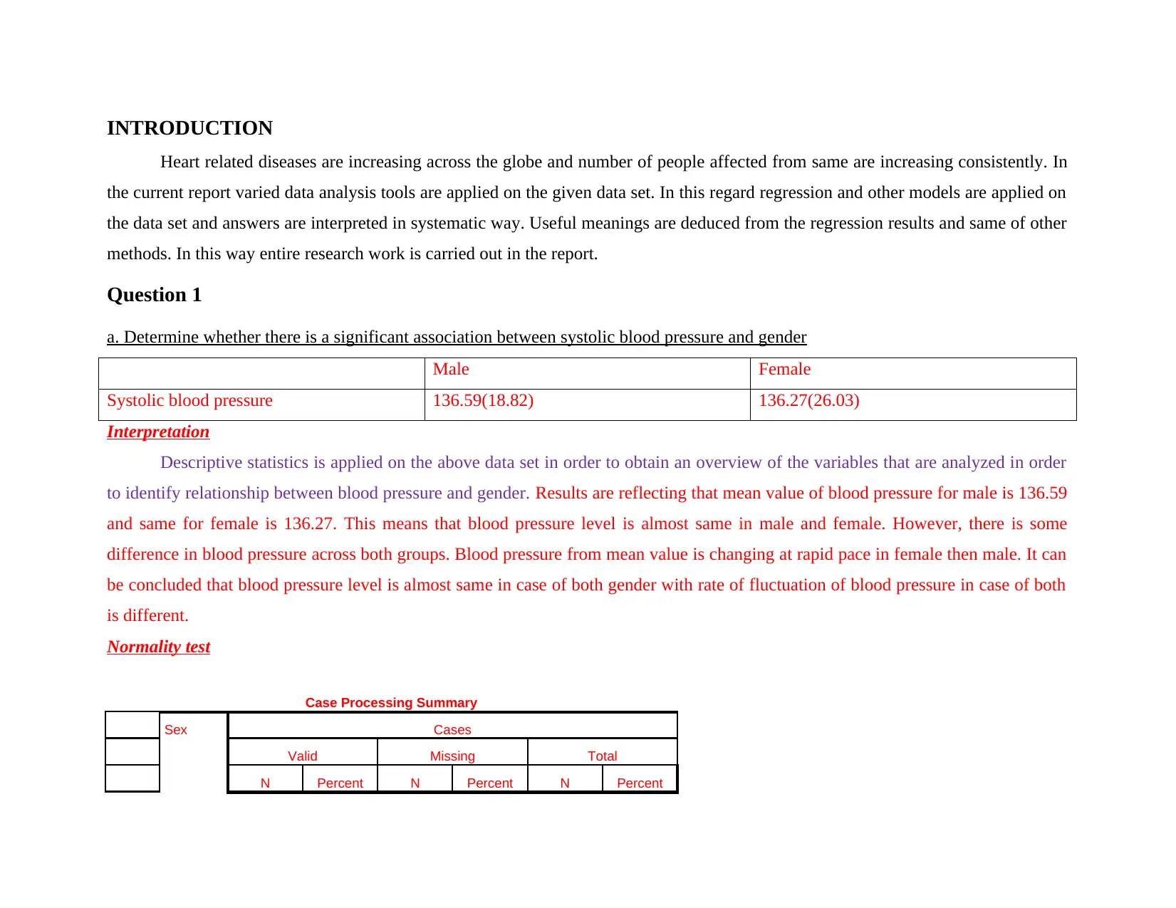
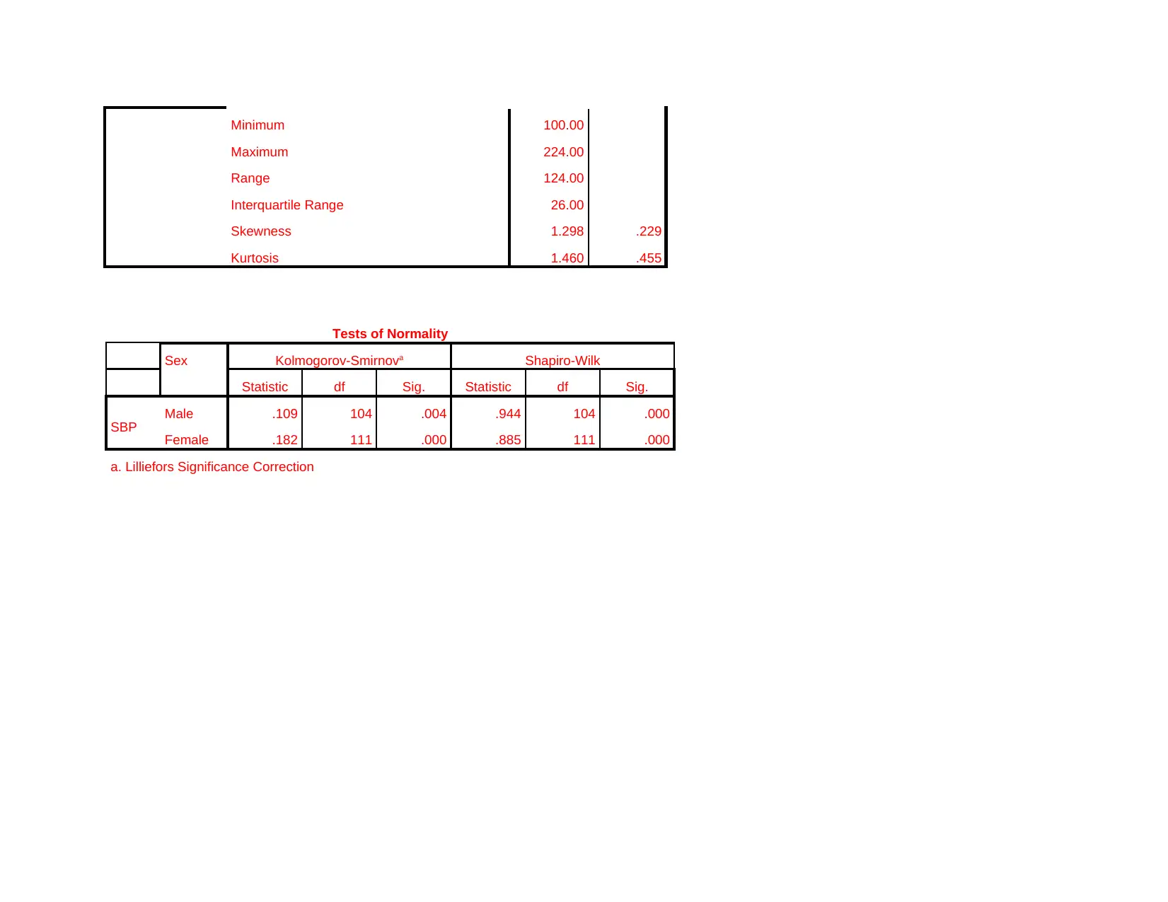
This report presents a comprehensive statistical analysis of blood pressure, employing various methods to investigate its relationships with different health factors. The analysis begins with descriptive statistics and tests for normality, exploring the association between systolic blood pressure and gender, as well as BMI categories. ANOVA and t-tests are used to determine significant differences in blood pressure across different groups. Further analysis delves into correlations between blood pressure, age, and cholesterol levels, followed by a linear regression analysis to assess the combined impact of these factors. The report also includes advanced statistical techniques such as Kaplan-Meier survival analysis, log-rank tests, and Cox regression to examine factors associated with coronary heart disease, providing a detailed interpretation of the results and their implications.

STATISTICS

TABLE OF CONTENTS
INTRODUCTION.......................................................................................................................................................................................3
Question 1....................................................................................................................................................................................................3
a. Determine whether there is a significant association between systolic blood pressure and gender....................................................3
b. Determine whether there is a significant association between systolic blood pressure and BMI category. Interpret your results.....5
c. Determine whether there is a significant association between systolic blood pressure and age as well as cholesterol......................6
Question 2..................................................................................................................................................................................................13
(a) Logistic regression...........................................................................................................................................................................13
Question 3..................................................................................................................................................................................................16
A. Carry out a Kaplan-Meier survival analysis.....................................................................................................................................16
(b) Construct a survival plot and conduct a hypothesis test using the log rank test..............................................................................17
© Cox regression...................................................................................................................................................................................20
...................................................................................................................................................................................................................23
(d) Significance of Cox proportional hazards model rather that logistic regression to determine which factors are associated with
coronary heart disease............................................................................................................................................................................24
CONCLUSION..........................................................................................................................................................................................24

INTRODUCTION
Heart related diseases are increasing across the globe and number of people affected from same are increasing consistently. In
the current report varied data analysis tools are applied on the given data set. In this regard regression and other models are applied on
the data set and answers are interpreted in systematic way. Useful meanings are deduced from the regression results and same of other
methods. In this way entire research work is carried out in the report.
Question 1
a. Determine whether there is a significant association between systolic blood pressure and gender
Male Female
Systolic blood pressure 136.59(18.82) 136.27(26.03)
Interpretation
Descriptive statistics is applied on the above data set in order to obtain an overview of the variables that are analyzed in order
to identify relationship between blood pressure and gender. Results are reflecting that mean value of blood pressure for male is 136.59
and same for female is 136.27. This means that blood pressure level is almost same in male and female. However, there is some
difference in blood pressure across both groups. Blood pressure from mean value is changing at rapid pace in female then male. It can
be concluded that blood pressure level is almost same in case of both gender with rate of fluctuation of blood pressure in case of both
is different.
Normality test
Case Processing Summary
Sex Cases
Valid Missing Total
N Percent N Percent N Percent

SBP Male 104 100.0% 0 0.0% 104 100.0%
Female 111 100.0% 0 0.0% 111 100.0%
Descriptives
Sex Statistic Std. Error
SBP
Male
Mean 136.5962 1.84624
95% Confidence Interval for
Mean
Lower Bound 132.9346
Upper Bound 140.2577
5% Trimmed Mean 135.6197
Median 134.5000
Variance 354.496
Std. Deviation 18.82805
Minimum 98.00
Maximum 210.00
Range 112.00
Interquartile Range 21.50
Skewness .993 .237
Kurtosis 2.278 .469
Female Mean 136.2703 2.47079
95% Confidence Interval for
Mean
Lower Bound 131.3737
Upper Bound 141.1668
5% Trimmed Mean 134.3008
Median 130.0000
Variance 677.635
Std. Deviation 26.03143

Minimum 100.00
Maximum 224.00
Range 124.00
Interquartile Range 26.00
Skewness 1.298 .229
Kurtosis 1.460 .455
Tests of Normality
Sex Kolmogorov-Smirnova Shapiro-Wilk
Statistic df Sig. Statistic df Sig.
SBP Male .109 104 .004 .944 104 .000
Female .182 111 .000 .885 111 .000
a. Lilliefors Significance Correction

Interpretation
Results are reflecting that data is not normally distributed. Significance value of Shapiro Wilk test is 0.00<0.05 which means
that data is not normally distributed. Histogram chart is prepared as part of normality test and it can be observed that in case of male
there is normality in the data to some extent as curve is bell shaped but not properly shaped. In case of female category histogram is
clearly reflecting that curve is not bell shaped. Thus, it can be said that data is not normally distributed as reflected by Shapiro wilk
test.
H0: There is no significant mean difference between gender and blood pressure.
H1: There is significant mean difference between gender and blood pressure.
Group Statistics
Sex N Mean Std. Deviation Std. Error Mean
SBP Male 104 136.5962 18.82805 1.84624
Female 111 136.2703 26.03143 2.47079
Independent Samples Test
Levene's Test for Equality of
Variances
t-test for Equality of Means
F Sig. t df Sig. (2-
tailed)
Mean
Difference
Std. Error
Difference
95% Confidence Interval of
the Difference
Lower Upper
SBP
Equal variances
assumed 6.391 .012 .105 213 .917 .32588 3.11614 -5.81653 6.46830
Equal variances not
assumed .106 200.406 .916 .32588 3.08439 -5.75613 6.40790

Interpretation
In order to identify whether there is significant difference between gender and blood pressure variable independent T test are
applied on the given data set. Descriptive table is clearly indicating that for males statistics are (mean=136.59 and standard
deviation=18.82) and same for female is (mean=136.27 and standard deviation is 26.03). Other test statistic revealed in the table are
mean difference= 0.33 and 95% confidence interval value is -5.76 to 6.40. Degree of freedom is 200.40 and t statistic value is 0.106.
Degree of freedom reflects the number of values in the statistics that are allowed to vary for calculation purpose. Results are reflecting
that in the calculation only 200 values of the independent variables are allowed to very. Value of t statistic is Value of level of
significance for T test applied on variable is 0.106 and it reflect the departure of an estimated parameter from specific value. Value of
level of significance is 0.916>0.05 which means that there is no significant difference between gender and blood pressure. This
reflects that null hypothesis is accepted.
b. Determine whether there is a significant association between systolic blood pressure and BMI category. Interpret your results
Tests of Normality
BMIcat Kolmogorov-Smirnova Shapiro-Wilk
Statistic df Sig. Statistic df Sig.
SBP
Normal .151 92 .000 .876 92 .000
Overweight .153 96 .000 .893 96 .000
Obese .181 27 .023 .868 27 .003
a. Lilliefors Significance Correction
Assumptions

 There must be dependent variable in the data set in respect to hypothesis. In the present case dependent variable is blood
pressure. Independent variable consists of categorical variable which may be male or female etc. There must be independence of observations. There must be no outliers in the dataset. Data must not be normally distributed.
H0: There is no significant difference between mean value of systolic blood pressure and BMI category.
H1: There is significant difference between mean value of systolic blood pressure and BMI category.
ANOVA
SBP
Sum of Squares df Mean Square F Sig.
Between Groups 10678.517 2 5339.259 11.276 .000
Within Groups 100380.115 212 473.491
Total 111058.633 214
Post Hoc Tests
Multiple Comparisons
Dependent Variable: SBP
Tukey HSD
(I) BMIcat (J) BMIcat Mean Difference (I-
J)
Std. Error Sig. 95% Confidence Interval
Lower Bound Upper Bound
Normal Overweight -14.09239* 3.17472 .000 -21.5857 -6.5991

Obese -14.75443* 4.76270 .006 -25.9958 -3.5130
Overweight Normal 14.09239* 3.17472 .000 6.5991 21.5857
Obese -.66204 4.74014 .989 -11.8502 10.5261
Obese Normal 14.75443* 4.76270 .006 3.5130 25.9958
Overweight .66204 4.74014 .989 -10.5261 11.8502
*. The mean difference is significant at the 0.05 level.
Homogeneous Subsets
SBP
Tukey HSD
BMIcat N Subset for alpha = 0.05
1 2
Normal 92 128.2826
Overweight 96 142.3750
Obese 27 143.0370
Sig. 1.000 .987
Means for groups in homogeneous subsets are displayed.
a. Uses Harmonic Mean Sample Size = 51.437.
b. The group sizes are unequal. The harmonic mean of the
group sizes is used. Type I error levels are not guaranteed.
Interpretation

Results are reflecting that data is not normally distributed as value of level of significance is 0.00 and this means condition is
satisfied. Results revealed that there is significant difference between dependent and independent variables. One way ANNOVA test is
applied on the relevant data set and in outcome table it can be observed that value of level of significance is 0.000<0.005 which mean
we can accept alternative hypothesis that there is significant mean difference between body mass index and blood pressure. It can be
concluded that rate of variation of body mass index and blood pressure are quite different from each other. Tuckey test is clearly
reflecting that there is significant difference in blood pressure in case of patients that are observing normal and overweight. On other
hand, there is significant mean difference in blood pressure in case of patients that are observing obese and overweight.
c. Determine whether there is a significant association between systolic blood pressure and age as well as cholesterol
Tests of Normalityc,d,e
Ageinyears Kolmogorov-Smirnova Shapiro-Wilk
Statistic df Sig. Statistic df Sig.
SBP 32.00 .256 6 .200* .909 6 .432
33.00 .113 8 .200* .991 8 .996
34.00 .202 5 .200* .936 5 .638
35.00 .178 7 .200* .969 7 .891
36.00 .219 6 .200* .898 6 .362
37.00 .192 5 .200* .895 5 .384
38.00 .157 9 .200* .977 9 .947
39.00 .385 3 . .750 3 .000
40.00 .245 8 .174 .921 8 .435
41.00 .254 5 .200* .914 5 .492
42.00 .160 10 .200* .941 10 .568
43.00 .220 5 .200* .961 5 .812