BM7024 Quantitative Data Analysis: Local Store Credit Card Decision

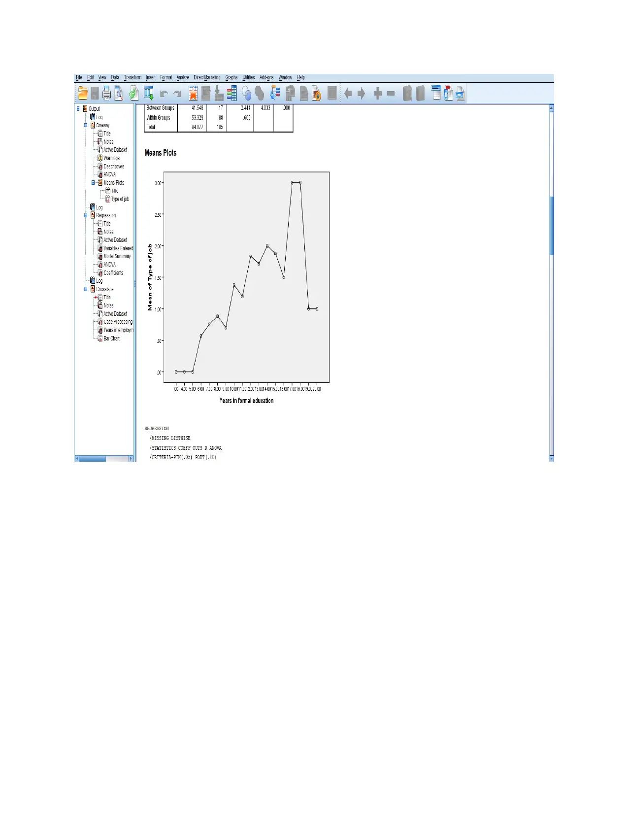
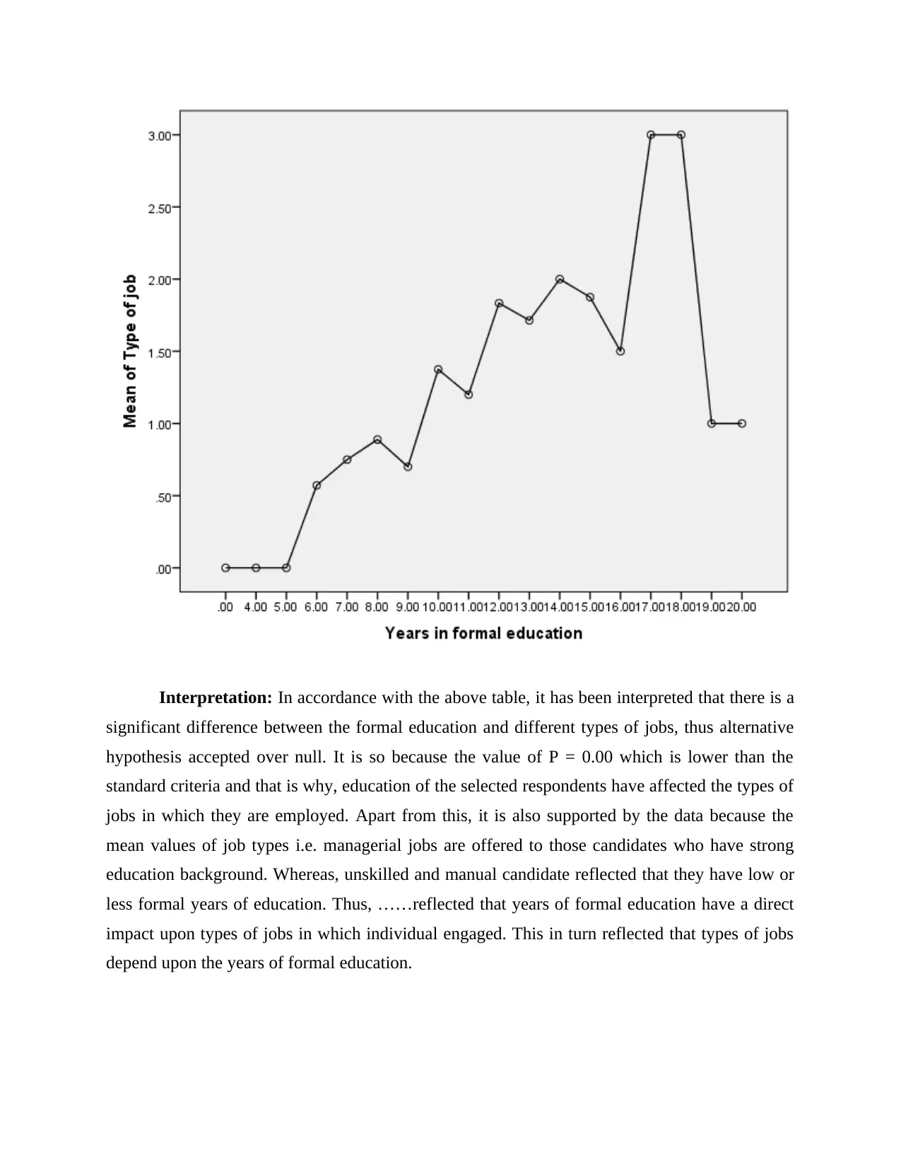
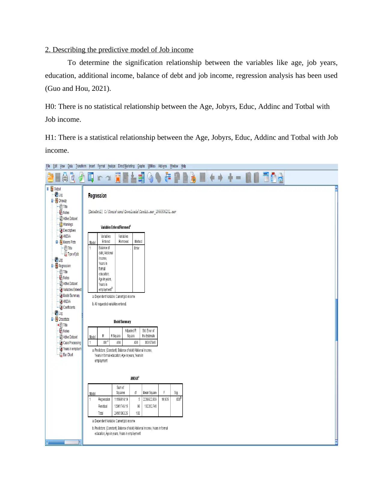
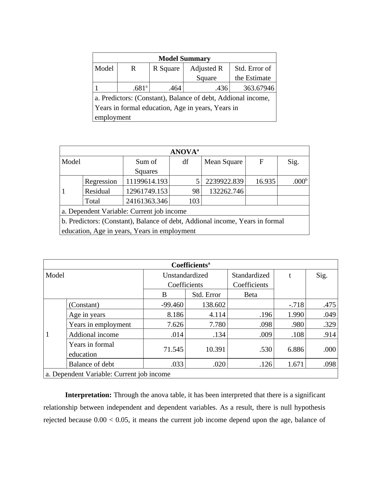
This report presents a quantitative data analysis conducted to assist a local store in making informed decisions regarding credit card issuance. The analysis employs inferential statistical tools, including one-way ANOVA and regression analysis, to explore relationships between variables such as formal education, job type, age, job years, income, and debt. The findings indicate a significant difference in formal education levels across different job types and a statistical relationship between job income and factors like age, education, and debt. Additionally, the report analyzes employment disparities between genders, revealing a lower representation of females in the workforce. Ultimately, the report provides valuable insights to aid the local store in its credit card issuance strategy, with additional resources available on Desklib.

Data Analysis – Quantitative

TABLE OF CONTENTS
INTRODUCTION...........................................................................................................................3
1. Presenting the significant difference in the years in formal education between the types of
job................................................................................................................................................3
2. Describing the predictive model of Job income......................................................................8
3. Analyzing employment is significantly lower for female compare to male respondents......10
CONCLUSION..............................................................................................................................14
REFERENCES..............................................................................................................................16

INTRODUCTION
Data analysis in quantitative study is all about analyzing the number based data that can
be used by various statistical techniques. The present report will highlight various inferential
statistic used in the present report to describe the relationship between the variables. The study is
based upon the case study of local store who is deciding whether store should or not issue a
credit card to their applicants.
1. Presenting the significant difference in the years in formal education between the types of job
In order to determine the significant differences, one –way anova as an inferential
statistical tool has been used that assist to examine the relationship between formal education and
type of jobs (Saeidi, Izanloo and Izanlou, 2020).
H0: (Null hypothesis): There is no significant difference between the years in formal education
between the type of jobs.
H1: (Alternative hypothesis): There is a significant difference between the years in formal
education between the type of jobs.

Descriptive
Type of job
N Mean Std.
Deviation
Std.
Error
95% Confidence Interval
for Mean
Minimum Maximum
Lower
Bound
Upper
Bound
.00 1 .0000 . . . . .00 .00
4.00 1 .0000 . . . . .00 .00
5.00 3 .0000 .00000 .00000 .0000 .0000 .00 .00
6.00 14 .5714 .85163 .22761 .0797 1.0631 .00 2.00
7.00 8 .7500 .70711 .25000 .1588 1.3412 .00 2.00
8.00 9 .8889 .92796 .30932 .1756 1.6022 .00 2.00
9.00 20 .7000 .80131 .17918 .3250 1.0750 .00 2.00

10.00 8 1.3750 .51755 .18298 .9423 1.8077 1.00 2.00
11.00 5 1.2000 .44721 .20000 .6447 1.7553 1.00 2.00
12.00 6 1.8333 .75277 .30732 1.0433 2.6233 1.00 3.00
13.00 7 1.7143 .95119 .35952 .8346 2.5940 1.00 3.00
14.00 5 2.0000 1.00000 .44721 .7583 3.2417 1.00 3.00
15.00 8 1.8750 .64087 .22658 1.3392 2.4108 1.00 3.00
16.00 6 1.5000 .83666 .34157 .6220 2.3780 1.00 3.00
17.00 1 3.0000 . . . . 3.00 3.00
18.00 2 3.0000 .00000 .00000 3.0000 3.0000 3.00 3.00
19.00 1 1.0000 . . . . 1.00 1.00
20.00 1 1.0000 . . . . 1.00 1.00
Total 106 1.1415 .95058 .09233 .9584 1.3246 .00 3.00
ANOVA
Type of job
Sum of
Squares
df Mean Square F Sig.
Between Groups 41.548 17 2.444 4.033 .000
Within Groups 53.329 88 .606
Total 94.877 105
Means Plots

Interpretation: In accordance with the above table, it has been interpreted that there is a
significant difference between the formal education and different types of jobs, thus alternative
hypothesis accepted over null. It is so because the value of P = 0.00 which is lower than the
standard criteria and that is why, education of the selected respondents have affected the types of
jobs in which they are employed. Apart from this, it is also supported by the data because the
mean values of job types i.e. managerial jobs are offered to those candidates who have strong
education background. Whereas, unskilled and manual candidate reflected that they have low or
less formal years of education. Thus, ……reflected that years of formal education have a direct
impact upon types of jobs in which individual engaged. This in turn reflected that types of jobs
depend upon the years of formal education.

2. Describing the predictive model of Job income
To determine the signification relationship between the variables like age, job years,
education, additional income, balance of debt and job income, regression analysis has been used
(Guo and Hou, 2021).
H0: There is no statistical relationship between the Age, Jobyrs, Educ, Addinc and Totbal with
Job income.
H1: There is a statistical relationship between the Age, Jobyrs, Educ, Addinc and Totbal with Job
income.

Model Summary
Model R R Square Adjusted R
Square
Std. Error of
the Estimate
1 .681a .464 .436 363.67946
a. Predictors: (Constant), Balance of debt, Addional income,
Years in formal education, Age in years, Years in
employment
ANOVAa
Model Sum of
Squares
df Mean Square F Sig.
1
Regression 11199614.193 5 2239922.839 16.935 .000b
Residual 12961749.153 98 132262.746
Total 24161363.346 103
a. Dependent Variable: Current job income
b. Predictors: (Constant), Balance of debt, Addional income, Years in formal
education, Age in years, Years in employment
Coefficientsa
Model Unstandardized
Coefficients
Standardized
Coefficients
t Sig.
B Std. Error Beta
1
(Constant) -99.460 138.602 -.718 .475
Age in years 8.186 4.114 .196 1.990 .049
Years in employment 7.626 7.780 .098 .980 .329
Addional income .014 .134 .009 .108 .914
Years in formal
education 71.545 10.391 .530 6.886 .000
Balance of debt .033 .020 .126 1.671 .098
a. Dependent Variable: Current job income
Interpretation: Through the anova table, it has been interpreted that there is a significant
relationship between independent and dependent variables. As a result, there is null hypothesis
rejected because 0.00 < 0.05, it means the current job income depend upon the age, balance of

debt, additional income and years of formal education as well as employment. Apart from this,
model summary table also reflected that if there is any change over the independent variables
then there is 46% change over job income. However, there is moderate association identified
over the variables because it has only 68% change over the current job income. Therefore, it has
been reflected by Wu and et.al., (2021) that individual income is depend upon different factors
which include age, formal education, additional income etc.
3. Analyzing employment is significantly lower for female compare to male respondents
To compare the categorical groups, cross-tab as an inferential statistic used in order to
generate the best outcomes and also determine whether years in employment is significantly
lower for female as compared to male respondents.
H0: There is no statistical difference between the mean value of employment and gender
H1: There is a statistical difference between the mean value of employment and gender

Case Processing Summary
Cases
Valid Missing Total
N Percent N Percent N Percent
Years in employment *
Gender 106 93.8% 7 6.2% 113 100.0%
Years in employment * Gender Crosstabulation
Count

Gender Total
Female Male
Years in
employment
.00 8 14 22
1.00 7 12 19
2.00 4 11 15
3.00 3 11 14
4.00 0 5 5
5.00 1 5 6
6.00 0 5 5
7.00 0 2 2
8.00 0 2 2
9.00 1 1 2
10.00 0 2 2
11.00 0 2 2
13.00 0 2 2
15.00 0 1 1
16.00 0 1 1
20.00 0 2 2
25.00 0 1 1
27.00 0 1 1
28.00 0 1 1
30.00 0 1 1
Total 24 82 106