MEM 355 Control System Design Project: Lateral Dynamics of Boeing 747

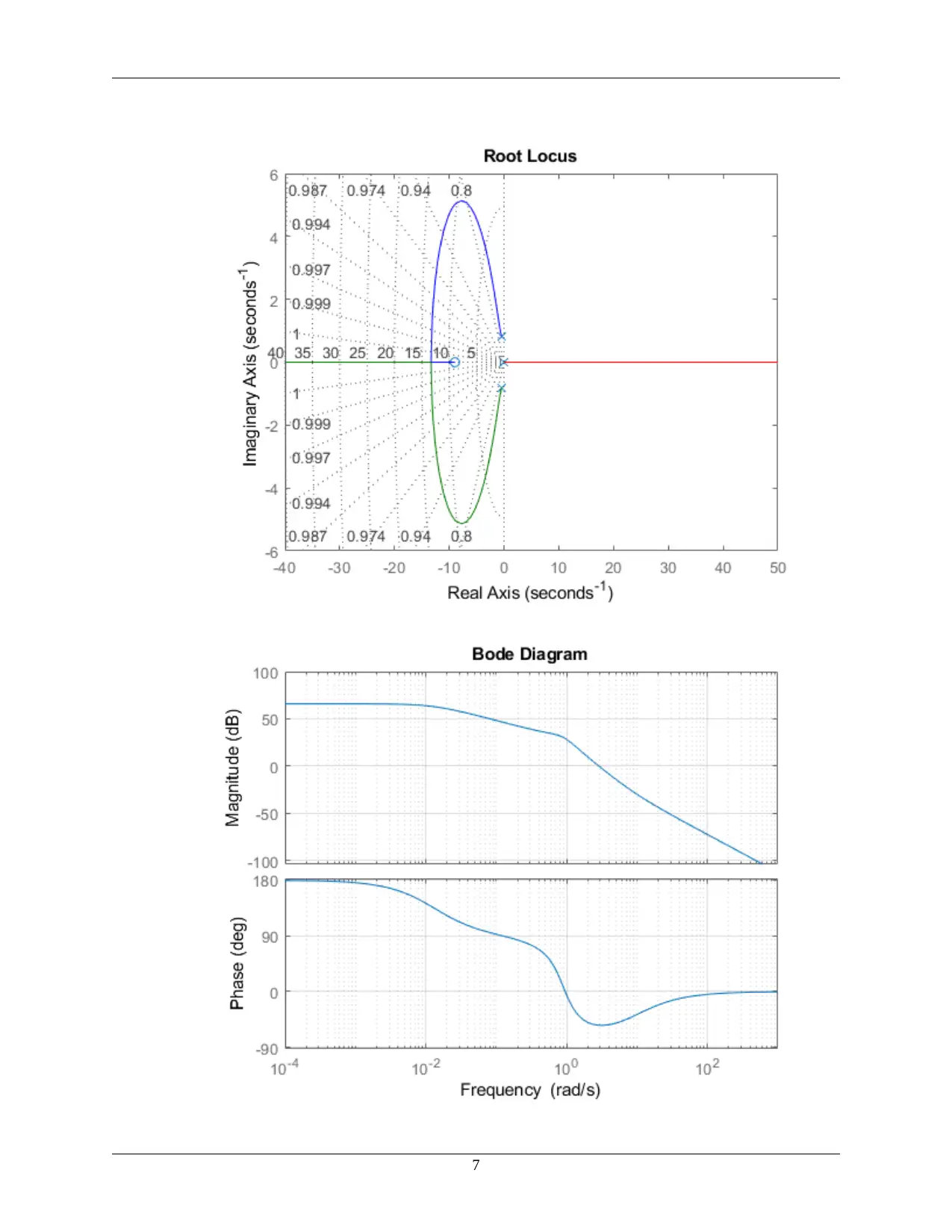
This project focuses on the design of a control system for the lateral dynamics of a Boeing 747, as part of the MEM 355 Control System Design course. The project utilizes MATLAB for computations, including the creation of state equations that incorporate the rudder actuator and a washout filter. The solution involves choosing specific closed-loop poles and obtaining a state feedback controller. The project analyzes the stability of the system using root locus and Bode plots. The design incorporates a rudder actuator and a washout filter to improve yaw rate control. Further analysis includes designing a compensator and an observer for the system. The results are presented with MATLAB code and plots, demonstrating the control system's performance and stability. The project aims to enhance understanding of control system design principles and their application to aircraft dynamics.

Table of Contents
Project MATLAB MEM 355 Control System Design ................................................................ 1
PART 1 ............................................................................................................................. 2
PART II ............................................................................................................................ 2
PART III ........................................................................................................................... 6
PART IV ........................................................................................................................... 8
Project MATLAB MEM 355 Control System De-
sign
%Lateral Dynamics of Boeing 747 (at mach 0.8 and 40,000ft)
%Beta-sideslip angle, r-yaw rate, p-roll rate, theta-roll angle
clear
close all
clc
%Creating the matrix for the aircraft
A=[-0.0558 -0.9968 0.0802 0.0415;0.598 -0.115 -0.0318 0;
-3.05 0.388 -0.465 0;0 0.0805 1 0];
B=[0.00729;-0.475;0.153;0];
[V,D]=eig(A);
disp('The eigenvalues are:')
disp(V);
disp('The eigenfunctions are:')
disp(D);
The eigenvalues are:
0.1994 - 0.1063i 0.1994 + 0.1063i -0.0172 + 0.0000i 0.0067 +
0.0000i
-0.0780 - 0.1333i -0.0780 + 0.1333i -0.0118 + 0.0000i 0.0404 +
0.0000i
-0.0165 + 0.6668i -0.0165 - 0.6668i -0.4895 + 0.0000i -0.0105 +
0.0000i
0.6930 + 0.0000i 0.6930 + 0.0000i 0.8717 + 0.0000i 0.9991 +
0.0000i
The eigenfunctions are:
-0.0329 + 0.9467i 0.0000 + 0.0000i 0.0000 + 0.0000i 0.0000 +
0.0000i
0.0000 + 0.0000i -0.0329 - 0.9467i 0.0000 + 0.0000i 0.0000 +
0.0000i
0.0000 + 0.0000i 0.0000 + 0.0000i -0.5627 + 0.0000i 0.0000 +
0.0000i
0.0000 + 0.0000i 0.0000 + 0.0000i 0.0000 + 0.0000i -0.0073 +
0.0000i
1

PART 1
%Constructing a state equation set with the rudder actuator and
washout
%filter
p=[-0.0051,-0.468,-0.279+0.628i,0.279+0.628i]; %closed loop poles
defr=place(A,B,p);
%Obtaining a state feedback controller to achieve those poles
p_or=eig(A-B*defr); %retains the original poles
Warning: A complex gain matrix is required when the pole locations are
not
specified as complex conjugate pairs.
PART II
den=-abs(p_or)';
num=[1.106,9.89];
Gc=tf(num,den)
%Determine stability of the system
figure(1)
rlocus(Gc)
grid on
figure(2)
bode(Gc)
grid on
% The rudder actuator
disp('The rudder Actuator')
Gr=tf(10,[1 10])
disp('The rudder Actuator & Aircraft')
Gc1=Gr*Gc
% including the washout filter at the feedback loop
disp('The washout filter')
Gh=tf(0.5,[1 0.5])
%Finding the tf of the closed loop function
G_closed=feedback(Gc1,Gh);
figure(3)
rlocus(G_closed) %The outcome unstable
grid on
figure(4)
bode(G_closed)
grid on
Gc =
-1.106 s - 9.89
2

------------------------------------------
0.468 s^3 + 0.0051 s^2 + 0.6872 s + 0.6872
Continuous-time transfer function.
The rudder Actuator
Gr =
10
------
s + 10
Continuous-time transfer function.
The rudder Actuator & Aircraft
Gc1 =
-11.06 s - 98.9
----------------------------------------------------
0.468 s^4 + 4.685 s^3 + 0.7382 s^2 + 7.559 s + 6.872
Continuous-time transfer function.
The washout filter
Gh =
0.5
-------
s + 0.5
Continuous-time transfer function.
3

4

5

PART III
p2=[-0.0253, -2.34, -1.39+1.34i,-1.39-1.34i];
c=[0,0,0,1];
defr2=place(A,B,p2)
%Obtaining a state feedback controller to achieve those poles
p_orB=eig(A-B*defr2) %retains the original poles
den=-abs(p_orB)';
num=[5.53 49.5];
GcB=tf(num,den);
figure(5)
rlocus(GcB) %observer for the system
grid on
figure(6)
bode(GcB)
grid on
defr2 =
12.7251 -10.3657 -3.3136 0.1852
p_orB =
-2.3400 + 0.0000i
-1.3900 + 1.3400i
-1.3900 - 1.3400i
-0.0253 + 0.0000i
6

7

PART IV
... Compensator transfer function
L=place(A',c',p2)'
eig(A-L*c)
Ac=A-B*defr2-L*c;
Bc=L;
Cc=defr2;
Gcss=ss(Ac,Bc,Cc,0);
Gcw=tf(Gcss);
rt=zpk(Gcw)
% Defining the root locus of the compensator
figure(7)
rlocus(rt)
grid on
figure(8)
L =
-1.3005
-1.8512
6.7054
4.5095
ans =
-2.3400 + 0.0000i
-1.3900 + 1.3400i
-1.3900 - 1.3400i
-0.0253 + 0.0000i
rt =
-18.744 (s-2.351) (s+0.7137) (s+0.006711)
------------------------------------------
(s+2.727) (s+3.646) (s^2 + 3.282s + 9.264)
Continuous-time zero/pole/gain model.
8

9

PREFORMATTED
TEXT
bode(rt)
grid on
Published with MATLAB® R2018b
10