Analyzing Boeing & General Dynamics Stocks Using Statistics

This report provides a statistical analysis of Boeing (BA) and General Dynamics (GD) stock prices from July 2011 to July 2016, utilizing monthly adjusted closing prices obtained from Yahoo Finance. The analysis includes trend identification, return calculations, and summary statistics, along with Jarque-Bera tests to assess normality. A one-sample t-test evaluates if GD's average return differs from 2.8%, while an F-test compares the variances of BA and GD. An independent sample t-test determines if the average returns of both stocks are similar. The Capital Asset Pricing Model (CAPM) is applied to GD, calculating excess returns and market returns to assess risk, with a regression analysis providing a coefficient of determination. Desklib offers this and other solved assignments for students seeking study resources.

Running Head: STATISTICS FOR BUSINESS AND FINANCE
Statistics for Business and Finance
Name of the Student
Name of the University
Author Note

1SFFBSTATISTICS FOR BUSINESS AND FINANCE
Table of Contents
Introduction......................................................................................................................................2
Task A..............................................................................................................................................2
Part 2................................................................................................................................................4
Part a............................................................................................................................................4
Part b............................................................................................................................................6
Part c............................................................................................................................................6
Part 3................................................................................................................................................7
Part 4................................................................................................................................................8
Part 5................................................................................................................................................8
Part 6................................................................................................................................................9
Part 7................................................................................................................................................9
Part a............................................................................................................................................9
Part b..........................................................................................................................................11
Part c..........................................................................................................................................11
Part d..........................................................................................................................................12
Part 8..............................................................................................................................................12
Part 9..............................................................................................................................................12

2SFFBSTATISTICS FOR BUSINESS AND FINANCE
Introduction
In order to invest in stock one should be able to analyse the stocks. The decision to invest can be
taken can be taken after an analysis of the performance of the stock. The performance of a stock
can be evaluated from its returns. Here we have evaluated the stocks of Boeing (BA) and
General Dynamics (GD). The adjusted closing prices of the stock for the period 1st July 2011 to
1st July 2016 have been taken to compare the performance of the stocks (roll No 1 9552104). The
information on the stock prices have been collected from yahoo finance. Monthly data of the
stock prices have been taken into account. Further, for market portfolio S&P 500 and to calculate
excess return “interest rate on 10-year treasury note” have been used.
The decision to invest in a stock depends on performance of the stock.
Task A
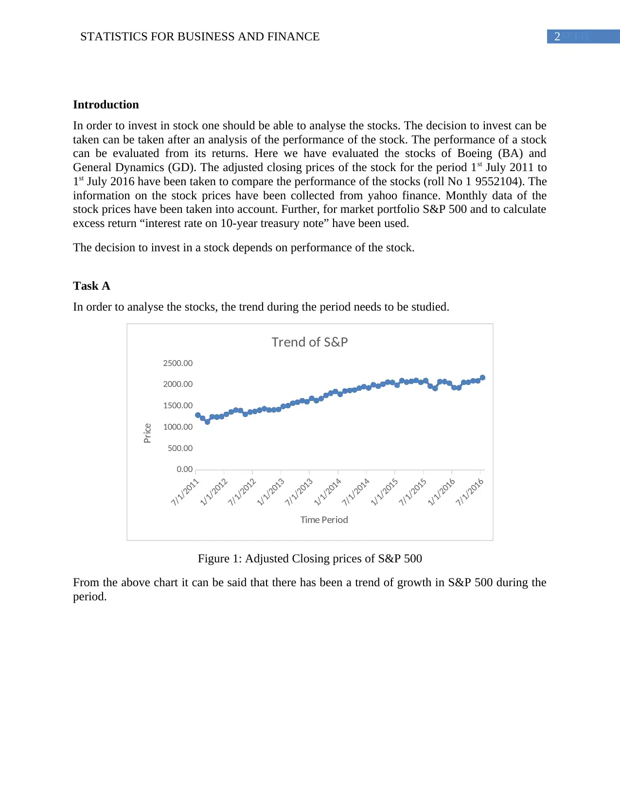
In order to analyse the stocks, the trend during the period needs to be studied.
7/1/2011
1/1/2012
7/1/2012
1/1/2013
7/1/2013
1/1/2014
7/1/2014
1/1/2015
7/1/2015
1/1/2016
7/1/2016
0.00
500.00
1000.00
1500.00
2000.00
2500.00
Trend of S&P
Time Period
Price
Figure 1: Adjusted Closing prices of S&P 500
From the above chart it can be said that there has been a trend of growth in S&P 500 during the
period.

3SFFBSTATISTICS FOR BUSINESS AND FINANCE
7/1/2011
1/1/2012
7/1/2012
1/1/2013
7/1/2013
1/1/2014
7/1/2014
1/1/2015
7/1/2015
1/1/2016
7/1/2016
0
20
40
60
80
100
120
140
160
Trend of Boeing
Time Period
Period
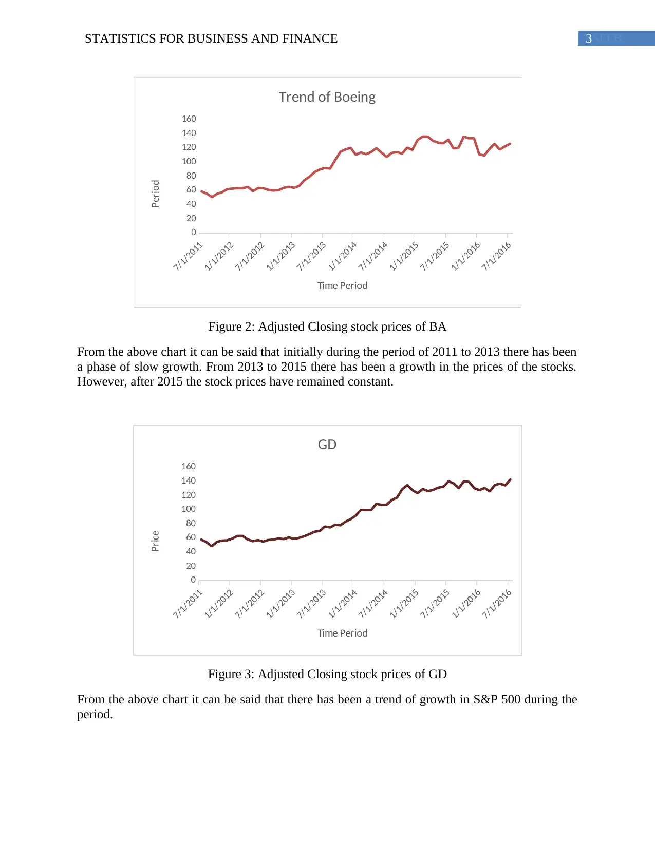
Figure 2: Adjusted Closing stock prices of BA
From the above chart it can be said that initially during the period of 2011 to 2013 there has been
a phase of slow growth. From 2013 to 2015 there has been a growth in the prices of the stocks.
However, after 2015 the stock prices have remained constant.
7/1/2011
1/1/2012
7/1/2012
1/1/2013
7/1/2013
1/1/2014
7/1/2014
1/1/2015
7/1/2015
1/1/2016
7/1/2016
0
20
40
60
80
100
120
140
160
GD
Time Period
Price
Figure 3: Adjusted Closing stock prices of GD
From the above chart it can be said that there has been a trend of growth in S&P 500 during the
period.

4SFFBSTATISTICS FOR BUSINESS AND FINANCE
Part 2
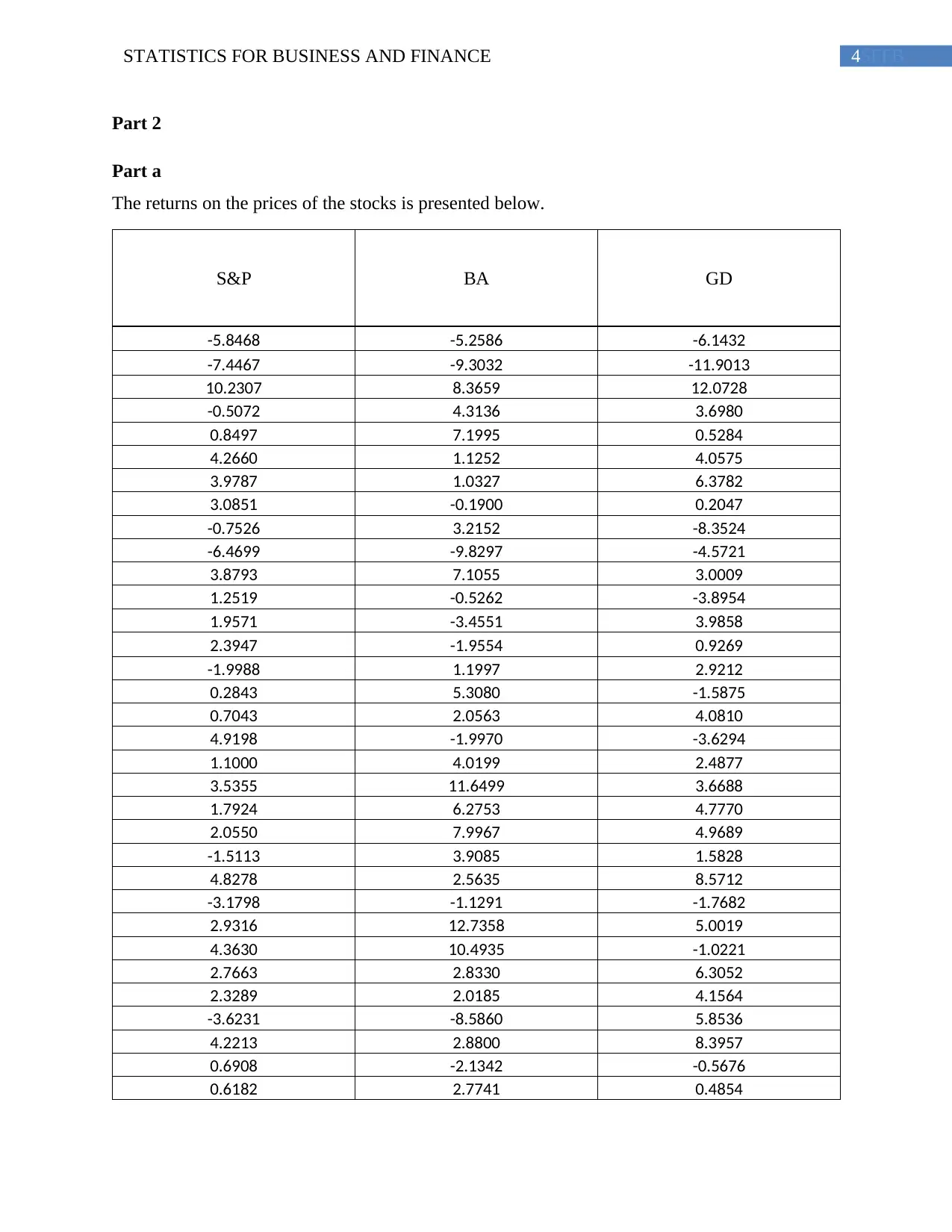
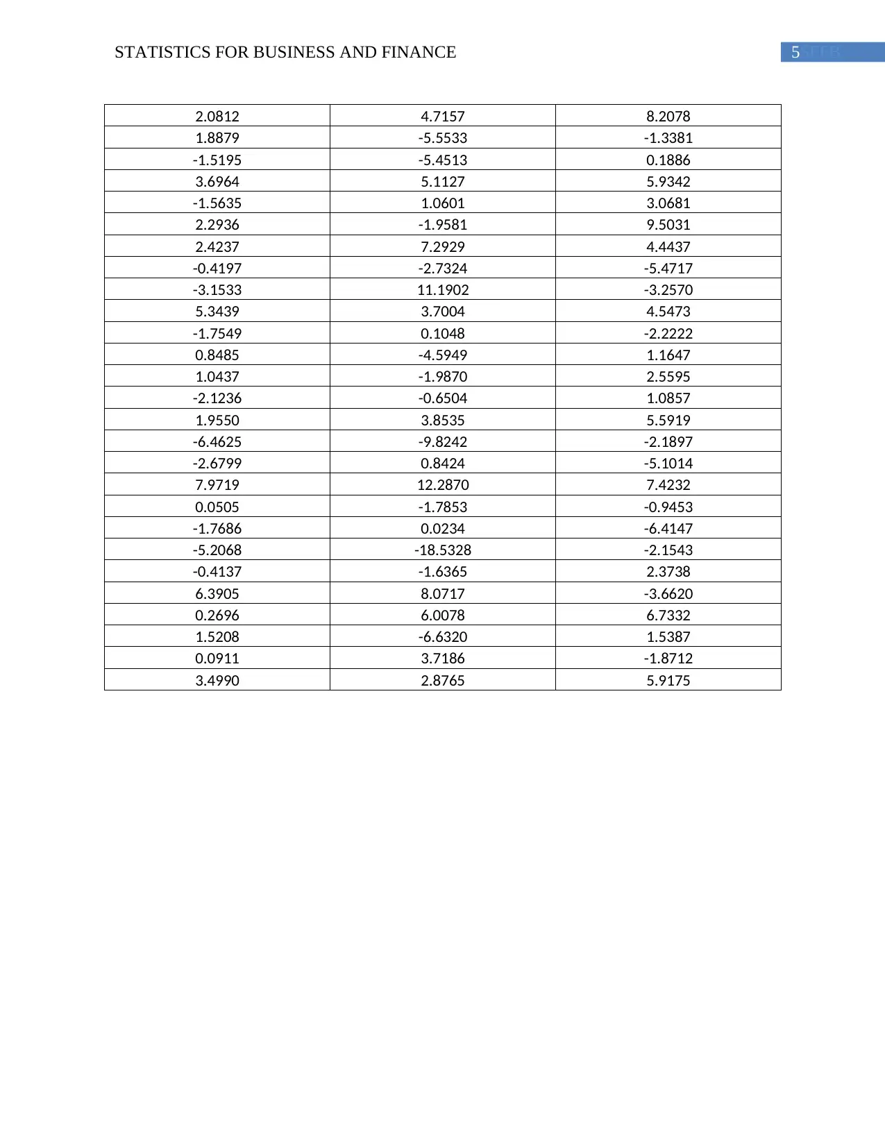
Part a
The returns on the prices of the stocks is presented below.
S&P BA GD
-5.8468 -5.2586 -6.1432
-7.4467 -9.3032 -11.9013
10.2307 8.3659 12.0728
-0.5072 4.3136 3.6980
0.8497 7.1995 0.5284
4.2660 1.1252 4.0575
3.9787 1.0327 6.3782
3.0851 -0.1900 0.2047
-0.7526 3.2152 -8.3524
-6.4699 -9.8297 -4.5721
3.8793 7.1055 3.0009
1.2519 -0.5262 -3.8954
1.9571 -3.4551 3.9858
2.3947 -1.9554 0.9269
-1.9988 1.1997 2.9212
0.2843 5.3080 -1.5875
0.7043 2.0563 4.0810
4.9198 -1.9970 -3.6294
1.1000 4.0199 2.4877
3.5355 11.6499 3.6688
1.7924 6.2753 4.7770
2.0550 7.9967 4.9689
-1.5113 3.9085 1.5828
4.8278 2.5635 8.5712
-3.1798 -1.1291 -1.7682
2.9316 12.7358 5.0019
4.3630 10.4935 -1.0221
2.7663 2.8330 6.3052
2.3289 2.0185 4.1564
-3.6231 -8.5860 5.8536
4.2213 2.8800 8.3957
0.6908 -2.1342 -0.5676
0.6182 2.7741 0.4854

5SFFBSTATISTICS FOR BUSINESS AND FINANCE
2.0812 4.7157 8.2078
1.8879 -5.5533 -1.3381
-1.5195 -5.4513 0.1886
3.6964 5.1127 5.9342
-1.5635 1.0601 3.0681
2.2936 -1.9581 9.5031
2.4237 7.2929 4.4437
-0.4197 -2.7324 -5.4717
-3.1533 11.1902 -3.2570
5.3439 3.7004 4.5473
-1.7549 0.1048 -2.2222
0.8485 -4.5949 1.1647
1.0437 -1.9870 2.5595
-2.1236 -0.6504 1.0857
1.9550 3.8535 5.5919
-6.4625 -9.8242 -2.1897
-2.6799 0.8424 -5.1014
7.9719 12.2870 7.4232
0.0505 -1.7853 -0.9453
-1.7686 0.0234 -6.4147
-5.2068 -18.5328 -2.1543
-0.4137 -1.6365 2.3738
6.3905 8.0717 -3.6620
0.2696 6.0078 6.7332
1.5208 -6.6320 1.5387
0.0911 3.7186 -1.8712
3.4990 2.8765 5.9175

6SFFBSTATISTICS FOR BUSINESS AND FINANCE
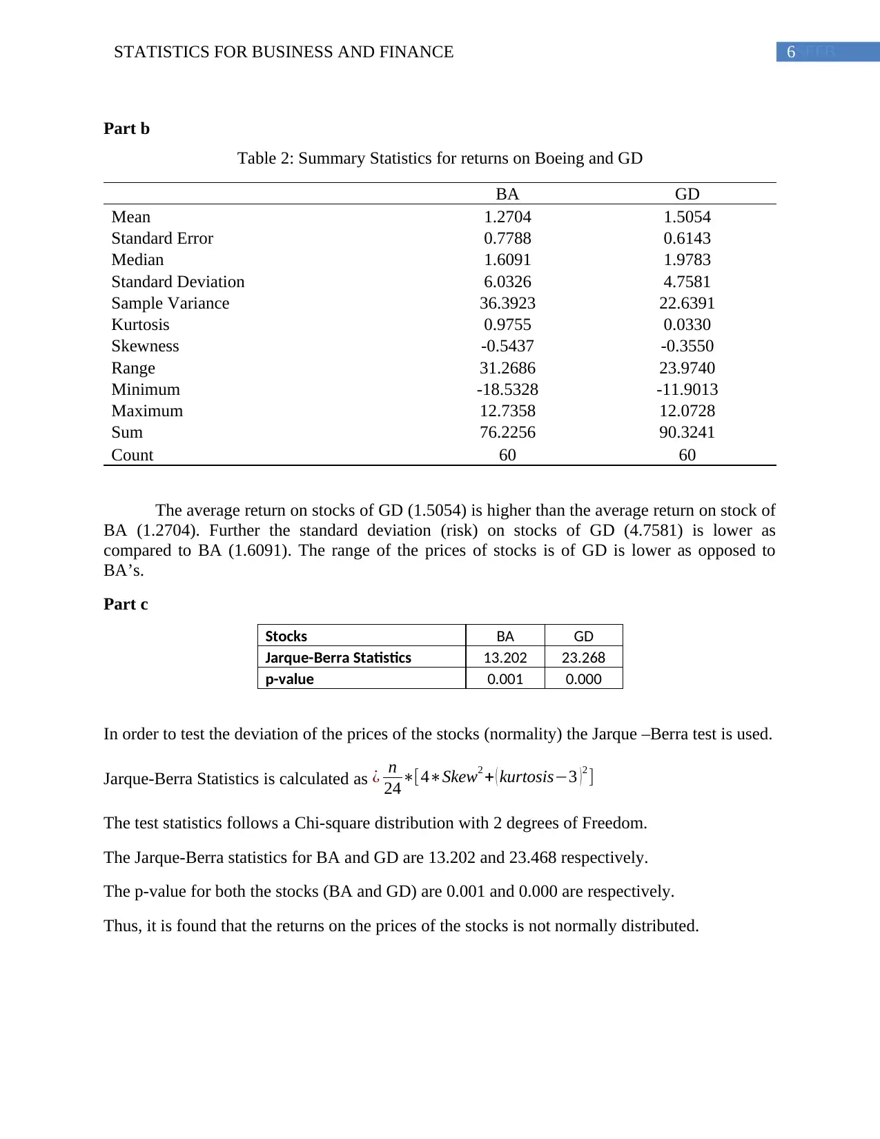
Part b
Table 2: Summary Statistics for returns on Boeing and GD
BA GD
Mean 1.2704 1.5054
Standard Error 0.7788 0.6143
Median 1.6091 1.9783
Standard Deviation 6.0326 4.7581
Sample Variance 36.3923 22.6391
Kurtosis 0.9755 0.0330
Skewness -0.5437 -0.3550
Range 31.2686 23.9740
Minimum -18.5328 -11.9013
Maximum 12.7358 12.0728
Sum 76.2256 90.3241
Count 60 60
The average return on stocks of GD (1.5054) is higher than the average return on stock of
BA (1.2704). Further the standard deviation (risk) on stocks of GD (4.7581) is lower as
compared to BA (1.6091). The range of the prices of stocks is of GD is lower as opposed to
BA’s.
Part c
Stocks BA GD
Jarque-Berra Statistics 13.202 23.268
p-value 0.001 0.000
In order to test the deviation of the prices of the stocks (normality) the Jarque –Berra test is used.
Jarque-Berra Statistics is calculated as ¿ n
24∗[4∗Skew2 + ( kurtosis−3 )2 ]
The test statistics follows a Chi-square distribution with 2 degrees of Freedom.
The Jarque-Berra statistics for BA and GD are 13.202 and 23.468 respectively.
The p-value for both the stocks (BA and GD) are 0.001 and 0.000 are respectively.
Thus, it is found that the returns on the prices of the stocks is not normally distributed.

7SFFBSTATISTICS FOR BUSINESS AND FINANCE
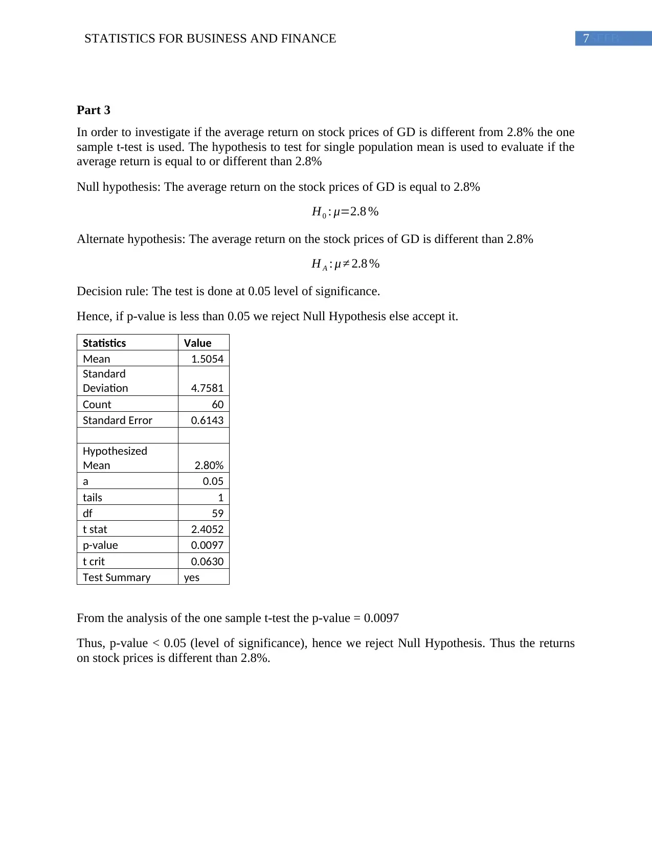
Part 3
In order to investigate if the average return on stock prices of GD is different from 2.8% the one
sample t-test is used. The hypothesis to test for single population mean is used to evaluate if the
average return is equal to or different than 2.8%
Null hypothesis: The average return on the stock prices of GD is equal to 2.8%
H0 : μ=2.8 %
Alternate hypothesis: The average return on the stock prices of GD is different than 2.8%
H A : μ ≠ 2.8 %
Decision rule: The test is done at 0.05 level of significance.
Hence, if p-value is less than 0.05 we reject Null Hypothesis else accept it.
Statistics Value
Mean 1.5054
Standard
Deviation 4.7581
Count 60
Standard Error 0.6143
Hypothesized
Mean 2.80%
a 0.05
tails 1
df 59
t stat 2.4052
p-value 0.0097
t crit 0.0630
Test Summary yes
From the analysis of the one sample t-test the p-value = 0.0097
Thus, p-value < 0.05 (level of significance), hence we reject Null Hypothesis. Thus the returns
on stock prices is different than 2.8%.

8SFFBSTATISTICS FOR BUSINESS AND FINANCE
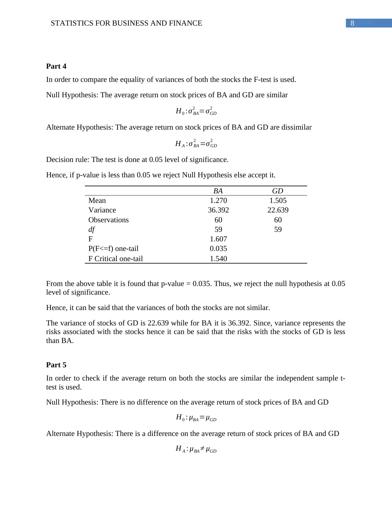
Part 4
In order to compare the equality of variances of both the stocks the F-test is used.
Null Hypothesis: The average return on stock prices of BA and GD are similar
H0 :σ BA
2 =σGD
2
Alternate Hypothesis: The average return on stock prices of BA and GD are dissimilar
H A :σ BA
2 =σGD
2
Decision rule: The test is done at 0.05 level of significance.
Hence, if p-value is less than 0.05 we reject Null Hypothesis else accept it.
BA GD
Mean 1.270 1.505
Variance 36.392 22.639
Observations 60 60
df 59 59
F 1.607
P(F<=f) one-tail 0.035
F Critical one-tail 1.540
From the above table it is found that p-value = 0.035. Thus, we reject the null hypothesis at 0.05
level of significance.
Hence, it can be said that the variances of both the stocks are not similar.
The variance of stocks of GD is 22.639 while for BA it is 36.392. Since, variance represents the
risks associated with the stocks hence it can be said that the risks with the stocks of GD is less
than BA.
Part 5
In order to check if the average return on both the stocks are similar the independent sample t-
test is used.
Null Hypothesis: There is no difference on the average return of stock prices of BA and GD
H0 : μBA =μGD
Alternate Hypothesis: There is a difference on the average return of stock prices of BA and GD
H A : μBA ≠ μGD

9SFFBSTATISTICS FOR BUSINESS AND FINANCE
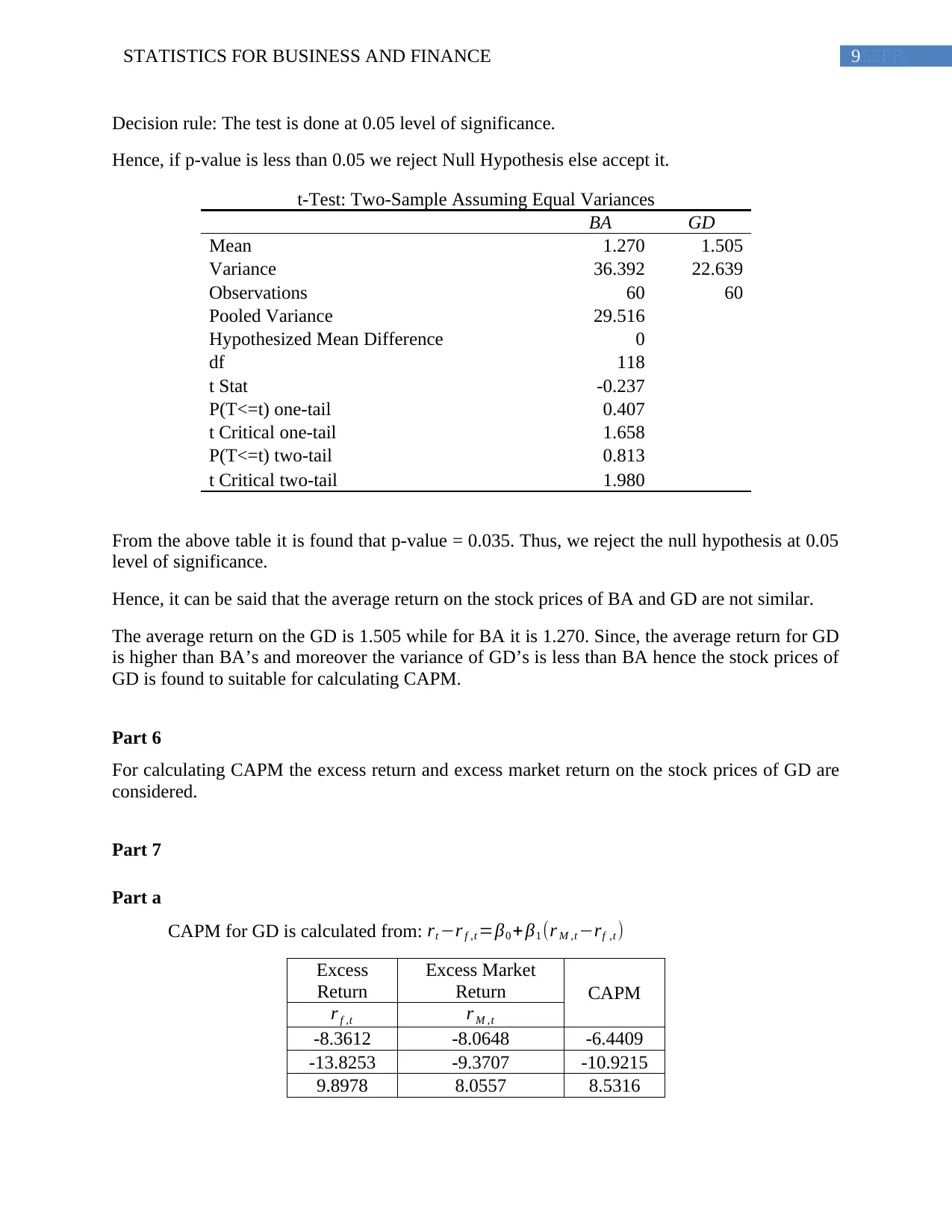
Decision rule: The test is done at 0.05 level of significance.
Hence, if p-value is less than 0.05 we reject Null Hypothesis else accept it.
t-Test: Two-Sample Assuming Equal Variances
BA GD
Mean 1.270 1.505
Variance 36.392 22.639
Observations 60 60
Pooled Variance 29.516
Hypothesized Mean Difference 0
df 118
t Stat -0.237
P(T<=t) one-tail 0.407
t Critical one-tail 1.658
P(T<=t) two-tail 0.813
t Critical two-tail 1.980
From the above table it is found that p-value = 0.035. Thus, we reject the null hypothesis at 0.05
level of significance.
Hence, it can be said that the average return on the stock prices of BA and GD are not similar.
The average return on the GD is 1.505 while for BA it is 1.270. Since, the average return for GD
is higher than BA’s and moreover the variance of GD’s is less than BA hence the stock prices of
GD is found to suitable for calculating CAPM.
Part 6
For calculating CAPM the excess return and excess market return on the stock prices of GD are
considered.
Part 7
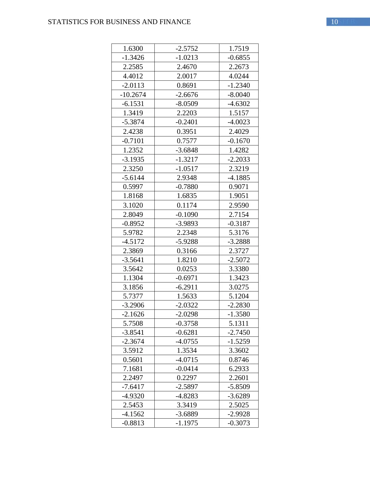
Part a
CAPM for GD is calculated from: rt −r f ,t =β0 + β1 (r M ,t −rf ,t )
Excess
Return
Excess Market
Return CAPM
r f ,t r M ,t
-8.3612 -8.0648 -6.4409
-13.8253 -9.3707 -10.9215
9.8978 8.0557 8.5316

10SFFBSTATISTICS FOR BUSINESS AND FINANCE
1.6300 -2.5752 1.7519
-1.3426 -1.0213 -0.6855
2.2585 2.4670 2.2673
4.4012 2.0017 4.0244
-2.0113 0.8691 -1.2340
-10.2674 -2.6676 -8.0040
-6.1531 -8.0509 -4.6302
1.3419 2.2203 1.5157
-5.3874 -0.2401 -4.0023
2.4238 0.3951 2.4029
-0.7101 0.7577 -0.1670
1.2352 -3.6848 1.4282
-3.1935 -1.3217 -2.2033
2.3250 -1.0517 2.3219
-5.6144 2.9348 -4.1885
0.5997 -0.7880 0.9071
1.8168 1.6835 1.9051
3.1020 0.1174 2.9590
2.8049 -0.1090 2.7154
-0.8952 -3.9893 -0.3187
5.9782 2.2348 5.3176
-4.5172 -5.9288 -3.2888
2.3869 0.3166 2.3727
-3.5641 1.8210 -2.5072
3.5642 0.0253 3.3380
1.1304 -0.6971 1.3423
3.1856 -6.2911 3.0275
5.7377 1.5633 5.1204
-3.2906 -2.0322 -2.2830
-2.1626 -2.0298 -1.3580
5.7508 -0.3758 5.1311
-3.8541 -0.6281 -2.7450
-2.3674 -4.0755 -1.5259
3.5912 1.3534 3.3602
0.5601 -4.0715 0.8746
7.1681 -0.0414 6.2933
2.2497 0.2297 2.2601
-7.6417 -2.5897 -5.8509
-4.9320 -4.8283 -3.6289
2.5453 3.3419 2.5025
-4.1562 -3.6889 -2.9928
-0.8813 -1.1975 -0.3073

11SFFBSTATISTICS FOR BUSINESS AND FINANCE
0.4645 -1.0513 0.7962
-1.2493 -4.4586 -0.6091
3.3869 -0.2500 3.1927
-4.3897 -8.6625 -3.1843
-7.1614 -4.7399 -5.4571
5.2722 5.8209 4.7386
-3.1633 -2.1675 -2.1786
-8.6837 -4.0376 -6.7054
-4.0853 -7.1378 -2.9346
0.6338 -2.1537 0.9351
-5.4480 4.6045 -4.0521
4.9142 -1.5494 4.4450
-0.2953 -0.3132 0.1732
-3.3592 -1.3969 -2.3392
4.4595 2.0410 4.0722
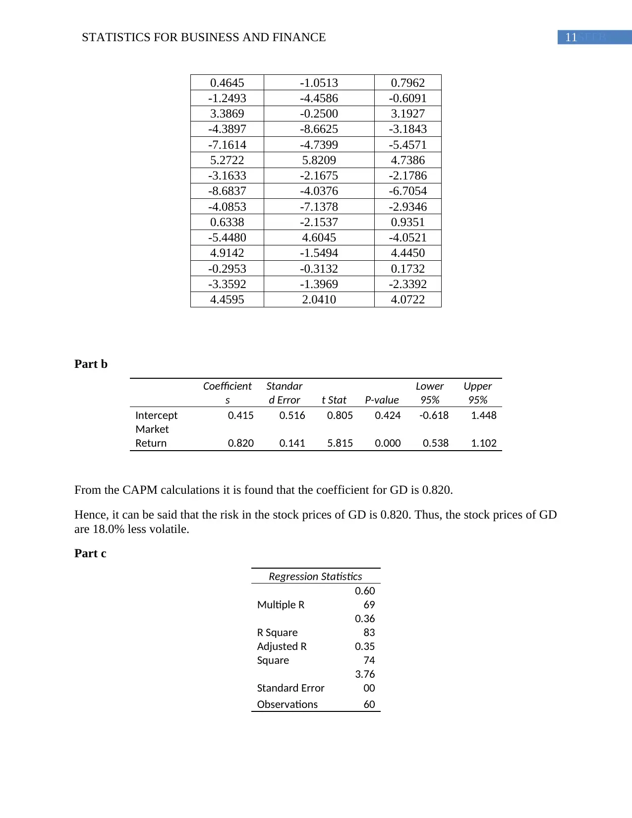
Part b
Coefficient
s
Standar
d Error t Stat P-value
Lower
95%
Upper
95%
Intercept 0.415 0.516 0.805 0.424 -0.618 1.448
Market
Return 0.820 0.141 5.815 0.000 0.538 1.102
From the CAPM calculations it is found that the coefficient for GD is 0.820.
Hence, it can be said that the risk in the stock prices of GD is 0.820. Thus, the stock prices of GD
are 18.0% less volatile.
Part c
Regression Statistics
Multiple R
0.60
69
R Square
0.36
83
Adjusted R
Square
0.35
74
Standard Error
3.76
00
Observations 60