Control Systems Engineering: Analyzing Boeing 747 Dynamics

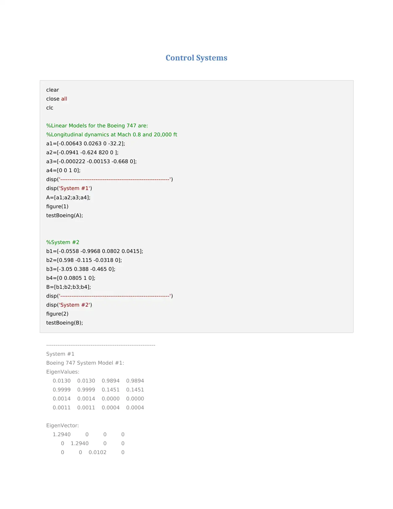
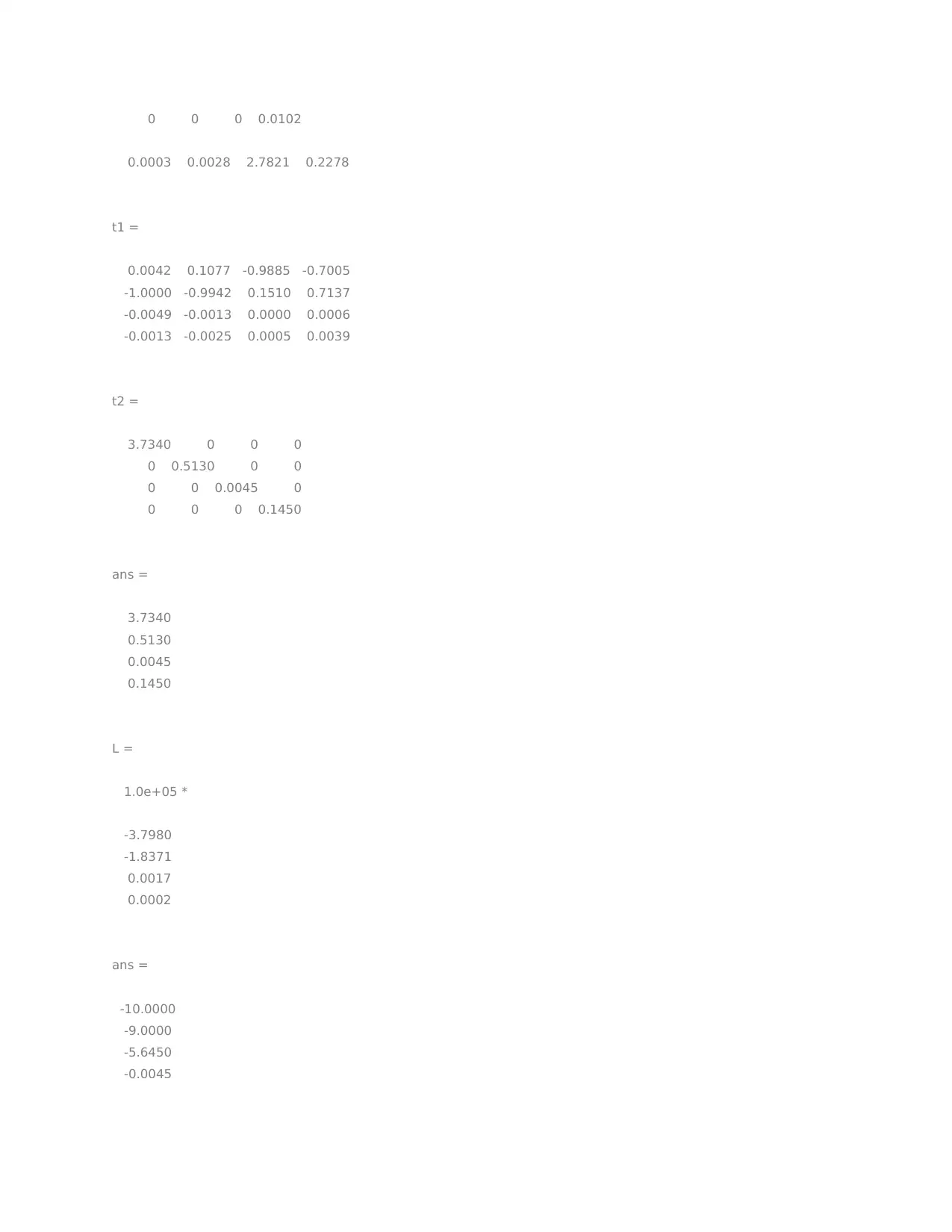
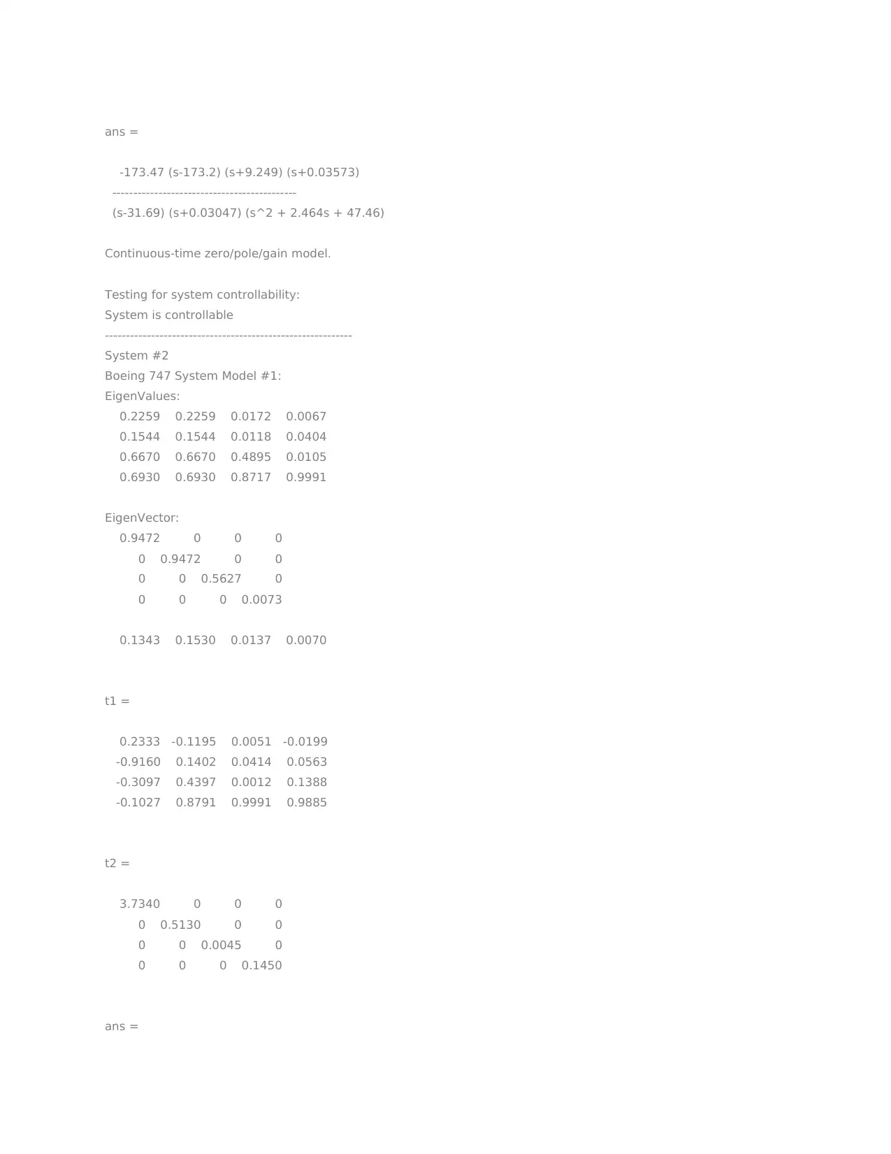
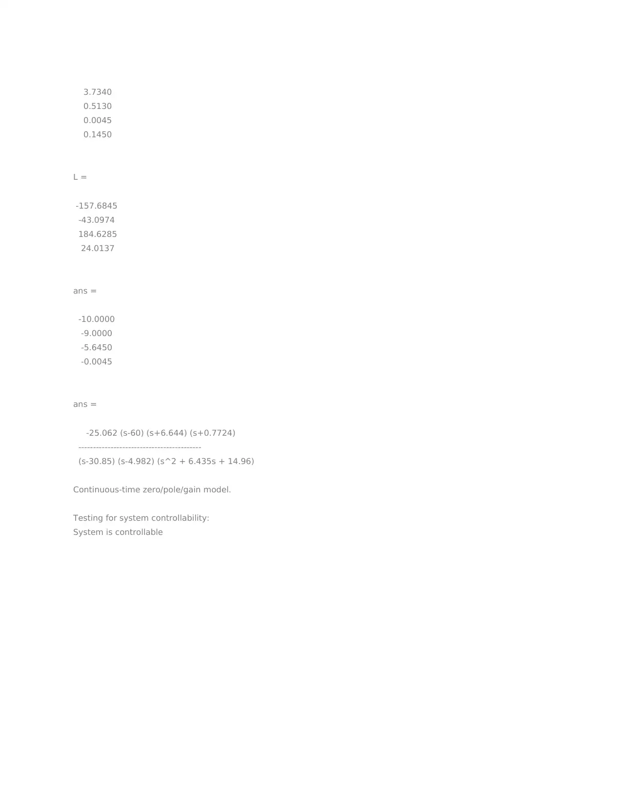
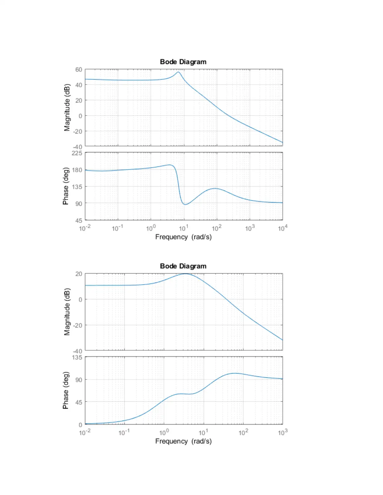
This assignment focuses on the analysis of control systems using linear models for the Boeing 747. It begins by defining linear models for the longitudinal dynamics of the Boeing 747 at Mach 0.8 and 20,000 ft, presenting two different system models (System #1 and System #2) represented by matri...Read More

Control Systems
clear
close all
clc
%Linear Models for the Boeing 747 are:
%Longitudinal dynamics at Mach 0.8 and 20,000 ft
a1=[-0.00643 0.0263 0 -32.2];
a2=[-0.0941 -0.624 820 0 ];
a3=[-0.000222 -0.00153 -0.668 0];
a4=[0 0 1 0];
disp('-----------------------------------------------------------')
disp('System #1')
A=[a1;a2;a3;a4];
figure(1)
testBoeing(A);
%System #2
b1=[-0.0558 -0.9968 0.0802 0.0415];
b2=[0.598 -0.115 -0.0318 0];
b3=[-3.05 0.388 -0.465 0];
b4=[0 0.0805 1 0];
B=[b1;b2;b3;b4];
disp('-----------------------------------------------------------')
disp('System #2')
figure(2)
testBoeing(B);
-----------------------------------------------------------
System #1
Boeing 747 System Model #1:
EigenValues:
0.0130 0.0130 0.9894 0.9894
0.9999 0.9999 0.1451 0.1451
0.0014 0.0014 0.0000 0.0000
0.0011 0.0011 0.0004 0.0004
EigenVector:
1.2940 0 0 0
0 1.2940 0 0
0 0 0.0102 0

0 0 0 0.0102
0.0003 0.0028 2.7821 0.2278
t1 =
0.0042 0.1077 -0.9885 -0.7005
-1.0000 -0.9942 0.1510 0.7137
-0.0049 -0.0013 0.0000 0.0006
-0.0013 -0.0025 0.0005 0.0039
t2 =
3.7340 0 0 0
0 0.5130 0 0
0 0 0.0045 0
0 0 0 0.1450
ans =
3.7340
0.5130
0.0045
0.1450
L =
1.0e+05 *
-3.7980
-1.8371
0.0017
0.0002
ans =
-10.0000
-9.0000
-5.6450
-0.0045

ans =
-173.47 (s-173.2) (s+9.249) (s+0.03573)
--------------------------------------------
(s-31.69) (s+0.03047) (s^2 + 2.464s + 47.46)
Continuous-time zero/pole/gain model.
Testing for system controllability:
System is controllable
-----------------------------------------------------------
System #2
Boeing 747 System Model #1:
EigenValues:
0.2259 0.2259 0.0172 0.0067
0.1544 0.1544 0.0118 0.0404
0.6670 0.6670 0.4895 0.0105
0.6930 0.6930 0.8717 0.9991
EigenVector:
0.9472 0 0 0
0 0.9472 0 0
0 0 0.5627 0
0 0 0 0.0073
0.1343 0.1530 0.0137 0.0070
t1 =
0.2333 -0.1195 0.0051 -0.0199
-0.9160 0.1402 0.0414 0.0563
-0.3097 0.4397 0.0012 0.1388
-0.1027 0.8791 0.9991 0.9885
t2 =
3.7340 0 0 0
0 0.5130 0 0
0 0 0.0045 0
0 0 0 0.1450
ans =

3.7340
0.5130
0.0045
0.1450
L =
-157.6845
-43.0974
184.6285
24.0137
ans =
-10.0000
-9.0000
-5.6450
-0.0045
ans =
-25.062 (s-60) (s+6.644) (s+0.7724)
------------------------------------------
(s-30.85) (s-4.982) (s^2 + 6.435s + 14.96)
Continuous-time zero/pole/gain model.
Testing for system controllability:
System is controllable