Statistical Analysis Homework: Bootstrap and Jackknife Techniques

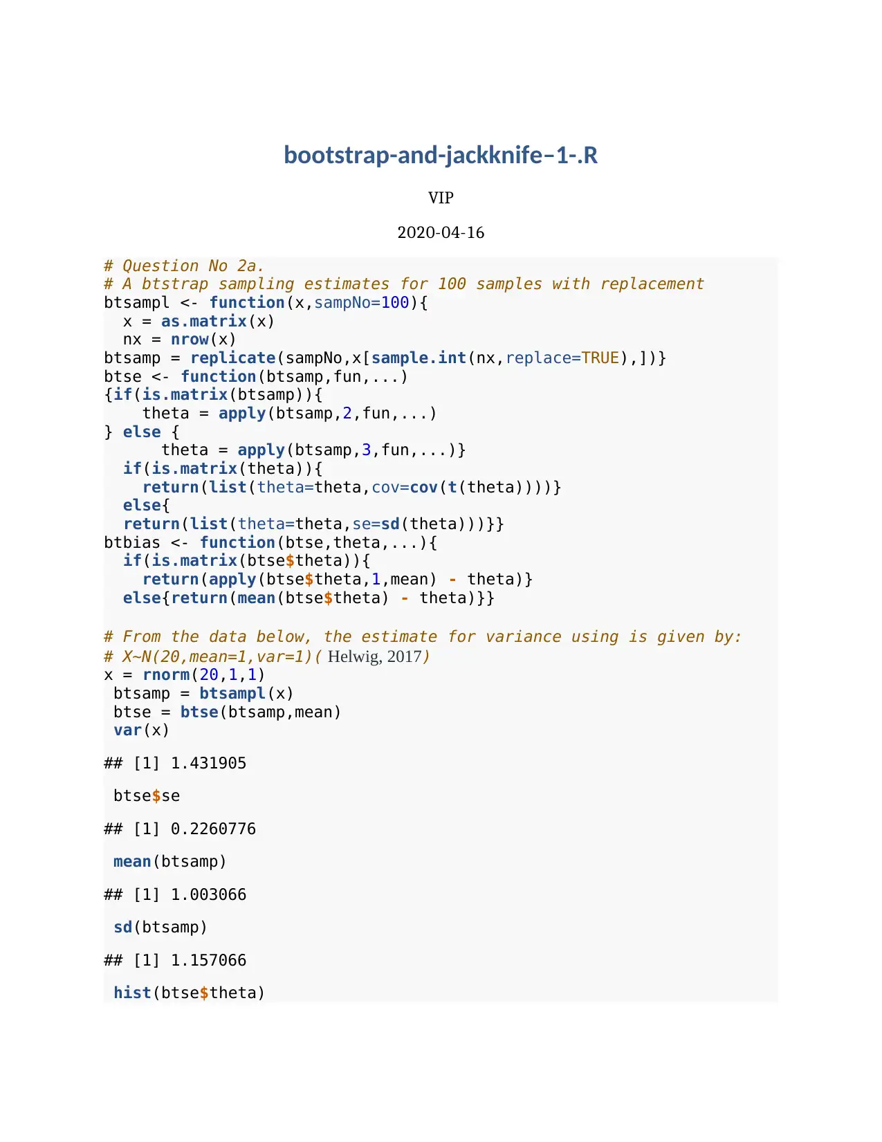
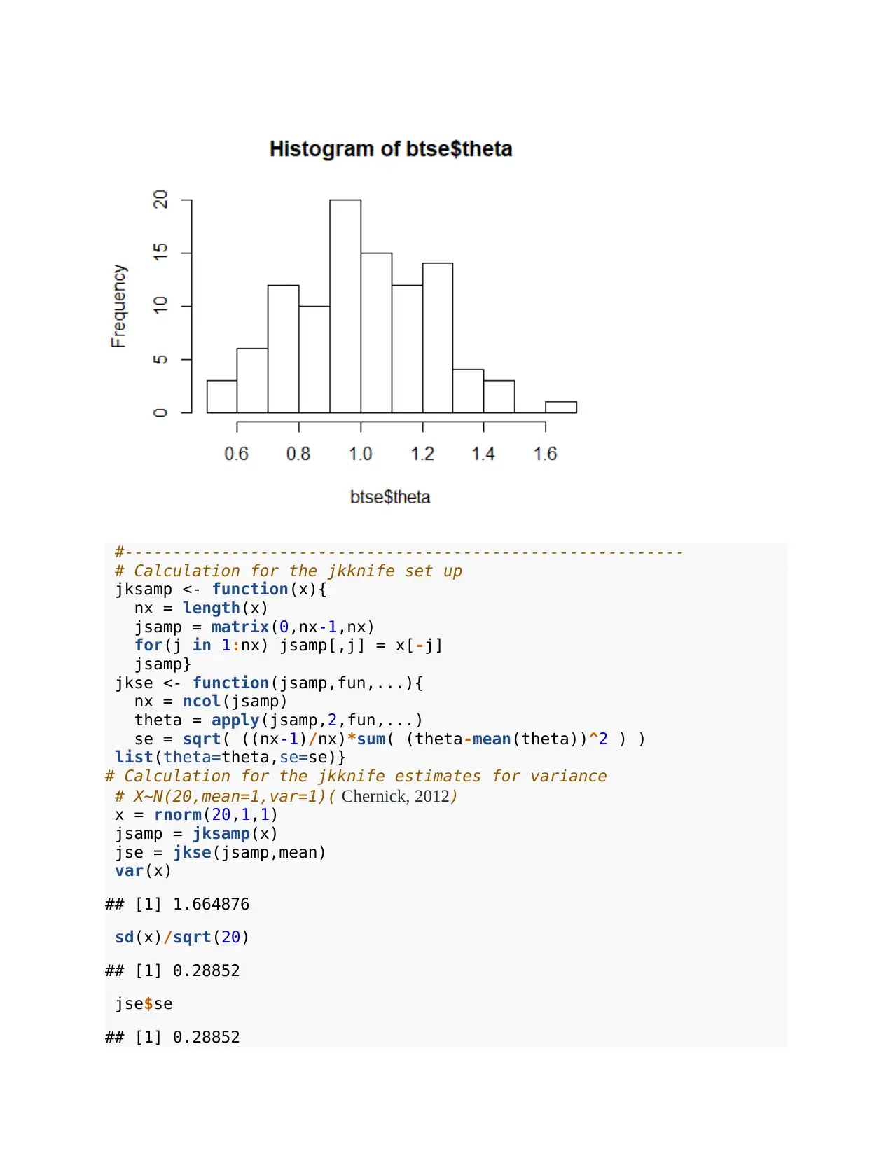
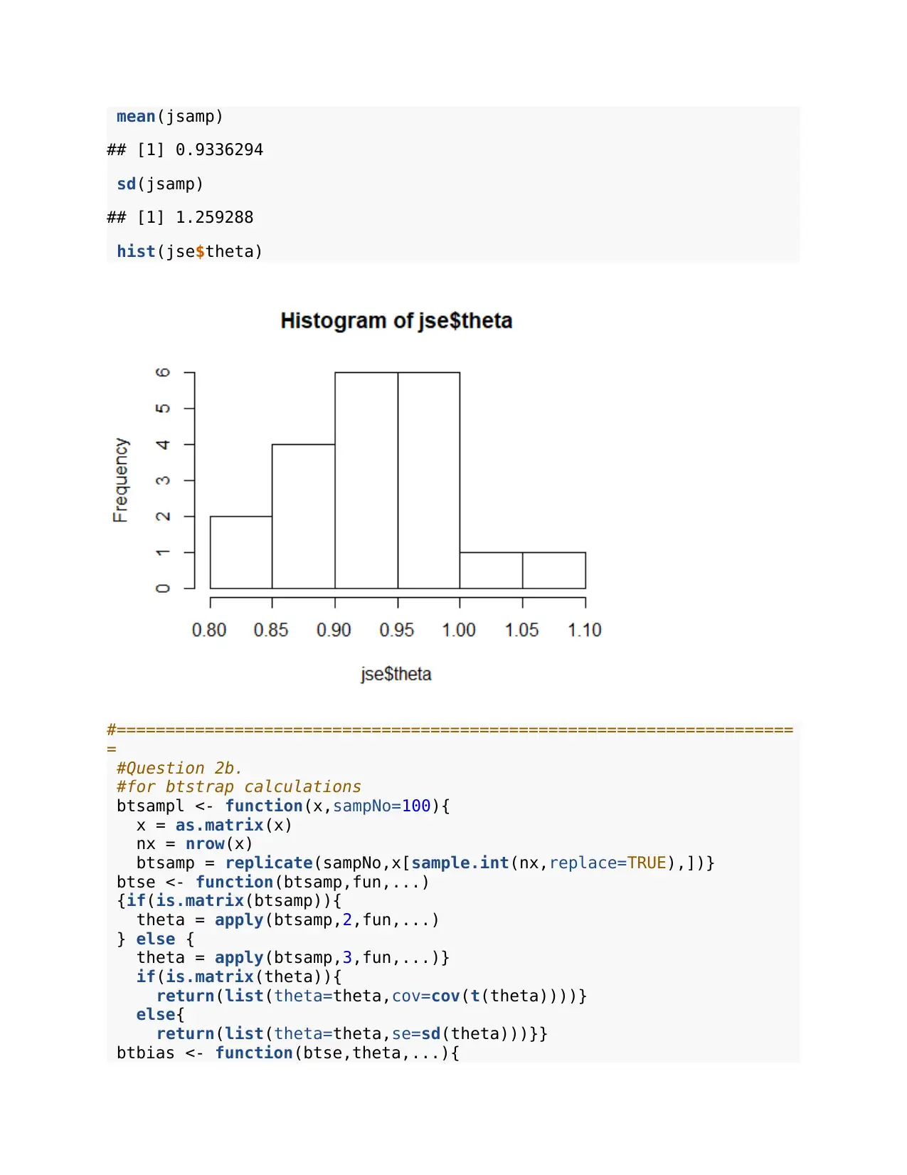
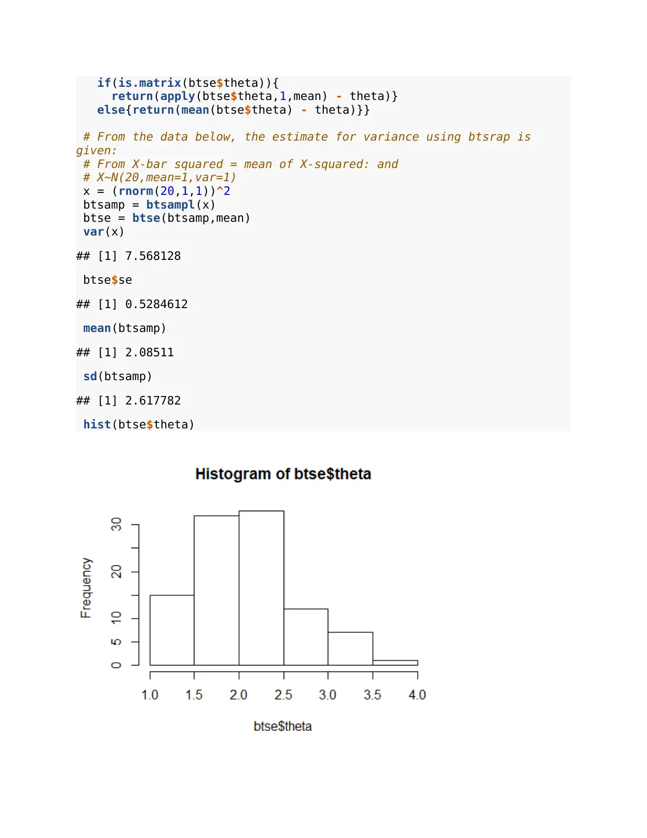
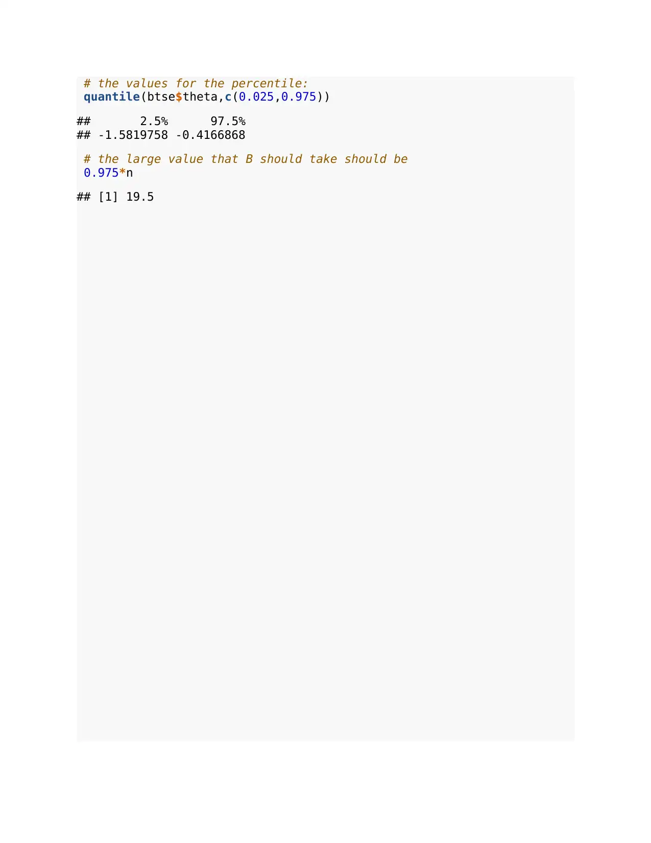
This document presents a comprehensive solution to a statistics homework assignment. The assignment focuses on applying bootstrap and jackknife methods for statistical analysis, including variance estimation and bias correction. The solution includes R code implementations of bootstrap sampling and jackknife estimation techniques, demonstrating their application to various datasets. The document covers the calculation of standard errors, confidence intervals, and the comparison of different estimation methods. The assignment explores both theoretical concepts and practical applications, providing a detailed analysis of the differences between bootstrap and jackknife methods in terms of their performance and accuracy. The solution also includes an analysis of confidence intervals and the use of these techniques in the context of different statistical distributions, providing a thorough understanding of these important statistical tools.

bootstrap-and-jackknife–1-.R
VIP
2020-04-16
# Question No 2a.
# A btstrap sampling estimates for 100 samples with replacement
btsampl <- function(x,sampNo=100){
x = as.matrix(x)
nx = nrow(x)
btsamp = replicate(sampNo,x[sample.int(nx,replace=TRUE),])}
btse <- function(btsamp,fun,...)
{if(is.matrix(btsamp)){
theta = apply(btsamp,2,fun,...)
} else {
theta = apply(btsamp,3,fun,...)}
if(is.matrix(theta)){
return(list(theta=theta,cov=cov(t(theta))))}
else{
return(list(theta=theta,se=sd(theta)))}}
btbias <- function(btse,theta,...){
if(is.matrix(btse$theta)){
return(apply(btse$theta,1,mean) - theta)}
else{return(mean(btse$theta) - theta)}}
# From the data below, the estimate for variance using is given by:
# X~N(20,mean=1,var=1)( Helwig, 2017)
x = rnorm(20,1,1)
btsamp = btsampl(x)
btse = btse(btsamp,mean)
var(x)
## [1] 1.431905
btse$se
## [1] 0.2260776
mean(btsamp)
## [1] 1.003066
sd(btsamp)
## [1] 1.157066
hist(btse$theta)

#----------------------------------------------------------
# Calculation for the jkknife set up
jksamp <- function(x){
nx = length(x)
jsamp = matrix(0,nx-1,nx)
for(j in 1:nx) jsamp[,j] = x[-j]
jsamp}
jkse <- function(jsamp,fun,...){
nx = ncol(jsamp)
theta = apply(jsamp,2,fun,...)
se = sqrt( ((nx-1)/nx)*sum( (theta-mean(theta))^2 ) )
list(theta=theta,se=se)}
# Calculation for the jkknife estimates for variance
# X~N(20,mean=1,var=1)( Chernick, 2012)
x = rnorm(20,1,1)
jsamp = jksamp(x)
jse = jkse(jsamp,mean)
var(x)
## [1] 1.664876
sd(x)/sqrt(20)
## [1] 0.28852
jse$se
## [1] 0.28852

mean(jsamp)
## [1] 0.9336294
sd(jsamp)
## [1] 1.259288
hist(jse$theta)
#=====================================================================
=
#Question 2b.
#for btstrap calculations
btsampl <- function(x,sampNo=100){
x = as.matrix(x)
nx = nrow(x)
btsamp = replicate(sampNo,x[sample.int(nx,replace=TRUE),])}
btse <- function(btsamp,fun,...)
{if(is.matrix(btsamp)){
theta = apply(btsamp,2,fun,...)
} else {
theta = apply(btsamp,3,fun,...)}
if(is.matrix(theta)){
return(list(theta=theta,cov=cov(t(theta))))}
else{
return(list(theta=theta,se=sd(theta)))}}
btbias <- function(btse,theta,...){

if(is.matrix(btse$theta)){
return(apply(btse$theta,1,mean) - theta)}
else{return(mean(btse$theta) - theta)}}
# From the data below, the estimate for variance using btsrap is
given:
# From X-bar squared = mean of X-squared: and
# X~N(20,mean=1,var=1)
x = (rnorm(20,1,1))^2
btsamp = btsampl(x)
btse = btse(btsamp,mean)
var(x)
## [1] 7.568128
btse$se
## [1] 0.5284612
mean(btsamp)
## [1] 2.08511
sd(btsamp)
## [1] 2.617782
hist(btse$theta)

#----------------------------------------------------------
# Calculation for the jkknife set up
jksamp <- function(x){
nx = length(x)
jsamp = matrix(0,nx-1,nx)
for(j in 1:nx) jsamp[,j] = x[-j]
jsamp}
jkse <- function(jsamp,fun,...){
nx = ncol(jsamp)
theta = apply(jsamp,2,fun,...)
se = sqrt( ((nx-1)/nx)*sum( (theta-mean(theta))^2 ) )
list(theta=theta,se=se)}
# Calculation for the jkknife estimates for variance
# X~N(20,mean=1,var=1)
x = (rnorm(20,1,1))^2
jsamp = jksamp(x)
jse = jkse(jsamp,mean)
var(x)
## [1] 5.193605
sd(x)/sqrt(20)
## [1] 0.5095883
jse$se
## [1] 0.5095883
mean(jsamp)
## [1] 1.802976
sd(jsamp)
## [1] 2.224173
hist(jse$theta)

# Explanation for the difference
# Although the values keep changing #
# since the data is random, #
# the estimators for mean X-bar are better than #
# those of X-bar squared because the errors are #
# are large for X-bar squared for one experiment the values were#
# method variance standardaError mean
standardDevation
#
# btstrap:Xbar 0.9351 0.2006 1.1069 0.9356
# :XbarSq 4.3905 0.4121 1.9996 2.1941
# jkknife:Xbar 0.8787 0.2096 1.3683 0.9149
# :XbarSq 11.4134 0.7553 2.7536 3.2972
#Question 3
# We take n=20 values of X and m=20 values of Y and,
# X~Norm with mean=2 and variance =1 while
# Y~Norm with mean=3 and variance =1
btsamp <- function(x,sampNo=100){
x = as.matrix(x)
nx = nrow(x)
btsamp = replicate(sampNo,x[sample.int(nx,replace=TRUE),])}
btse <- function(btsamp,fun,...){
if(is.matrix(btsamp)){
theta = apply(btsamp,2,fun,...)}
else {theta = apply(btsamp,3,fun,...)}
if(is.matrix(theta)){

return(list(theta=theta,cov=cov(t(theta))))}
else{
return(list(theta=theta,se=sd(theta)))}}
Bcafunc <- function(x,nbt,theta,...,alpha=0.05){
theta.hat = theta(x)
nx = length(x)
btse = btse(btsamp(x,nbt),theta,...)
jse = jkse(jksamp(x),theta,...)
z0 = qnorm(sum(btse$theta<theta.hat)/nbt)
a_top = sum((mean(jse$theta)-jse$theta)^3)
a_bot = 6*(((jse$se^2)*nx/(nx-1))^(3/2))
a_hat = a_top/a_bot
apha1 = pnorm(z0+(z0+qnorm(alpha))/(1-a_hat*(z0+qnorm(alpha))))
apha2 = pnorm(z0+(z0+qnorm(1-alpha))/(1-a_hat*(z0+qnorm(1-
alpha))))
confpoint = quantile(btse$theta,probs=c(apha1,apha2))
list(confpoint=confpoint,z0=z0,acc=a_hat,u=(jse$theta-theta.hat),
theta=btse$theta,se=btse$se)
}
x = rnorm(20,2,1)
y = rnorm(20,3,1)
z = cbind(x,y)
n=20
btsamp = btsamp(z)
fun = function(z) mean(z[,1]) - mean(z[,2])
fun
## function(z) mean(z[,1]) - mean(z[,2])
btse = btse(btsamp,fun)
fun(z)
## [1] -0.9109713
sqrt( (var(z[,1])+var(z[,2]))/nrow(z) )
## [1] 0.3026102
btse$se
## [1] 0.3265907
hist(btse$theta)

# The 95% confidence for M1-M2
c(mean(z)-qnorm(0.975)*sd(z)*sqrt((n-1)/n)/sqrt(n),
mean(z)-qnorm(0.025)*sd(z)*sqrt((n-1)/n)/sqrt(n))
## [1] 1.914715 2.812791
# Using the btstrap technique, the 95% confidence
fun(z) - 1.96*sqrt(var(btsamp))
## [1] -2.966136
fun(z) + 1.96*sqrt(var(btsamp))
## [1] 1.144193
# For the B btstraps needed for the 95% CI created above, we
calculate the interval using
btsampSE = apply(btsamp, 2, sd)*sqrt((n-1)/n) / sqrt(n)
theta = mean(z)
w = (btse$theta - theta) / btsampSE
confval = quantile(w, probs=c(0.025,0.975))
# a bootstrap t-table:
c(theta - confval[2]*btse$se, theta - confval[1]*btse$se)
## 97.5% 2.5%
## 6.744248 8.660356

# the values for the percentile:
quantile(btse$theta,c(0.025,0.975))
## 2.5% 97.5%
## -1.5819758 -0.4166868
# the large value that B should take should be
0.975*n
## [1] 19.5

References
Chernick, M. R. (2012). The jackknife: a resampling method with connections to the
bootstrap. Wiley Interdisciplinary Reviews: Computational Statistics, 4(2), 224-226.
Helwig, N. E. (2017). Bootstrap confidence intervals. Minneapolis and Saint Paul: University of
Minnesota (Twin Cities).