Brownian Dynamics Simulations of Polymers: A Physics Perspective

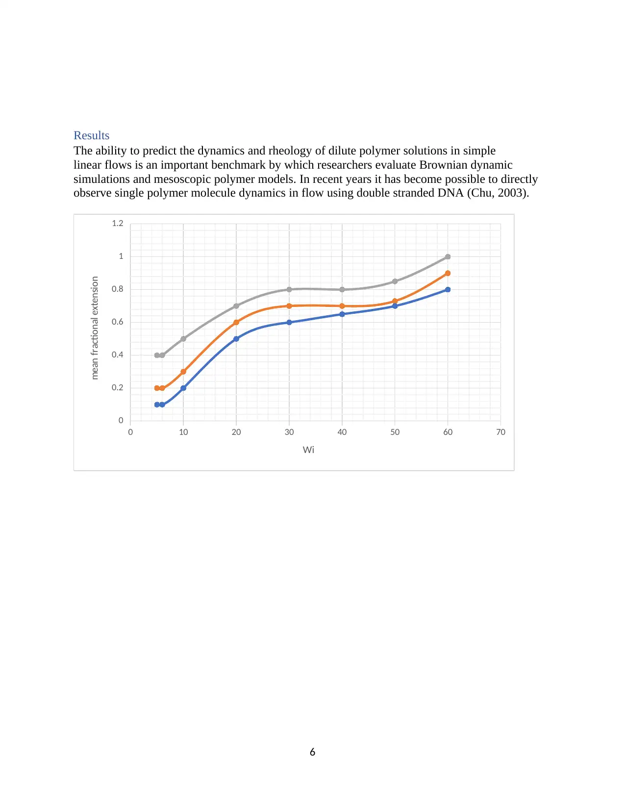
This report delves into the application of Brownian dynamics simulations for studying polymers, highlighting its advantage as a mesoscopic physics method where explicit solvent particles are replaced by a stochastic force. It discusses the basics of Brownian dynamics, including the Langevin equation and the incorporation of hydrodynamic interactions through tensors. The report also explores various polymer models used in Brownian dynamics, such as freely-jointed bead-rod and bead-spring chains, and presents results demonstrating the technique's ability to predict the dynamics and rheology of dilute polymer solutions. The conclusion emphasizes the power of Brownian dynamics in simulating nonequilibrium dynamics of polymers and other soft matter, noting its advancements in treating molecules in confined spaces and the importance of quantitative comparisons to single molecule DNA experiments. The document includes a bibliography of cited works.

BROWNIAN DYNAMICS SIMULATIONS OF POLYMERS
Contents
1

Abstract.......................................................................................................................................................3
Introduction.................................................................................................................................................4
Methodology...............................................................................................................................................5
Results.........................................................................................................................................................6
Conclusion...................................................................................................................................................7
Bibliography................................................................................................................................................8
2

Abstract
The Brownian dynamics simulation method is a mesoscopic physic method were the explicit
solvent particles are substituted by a stochastic force. This method is advantageous because there
is wide separation especially on time scale among the fast motion solvent particles/molecules
and the further slow motion of polymers. The capability of coarse graining
out the rapid means of solvent enables the simulation of wide time scales as compared to
molecular dynamics simulation. At the pivotal point of Brownian dynamics simulation always
will be a stochastic differential equation that will be integrated with time in order to generate
trajectories of particles/molecules. Brownian dynamics simulations is particularly suited to study
the structure and also rheology of complex fluids in hydrodynamic flows and
other nonequilibrium situations
3

Introduction
.
Basic Brownian Dynamics
The method of Brownian dynamics simulates the dynamics of particles that always
undergo Brownian motion. Due to small mass of the molecules, the inertia force is
neglected. By using Newton’s Second Law for particle [F = ma ] and neglecting the inertia force
will approximate the total force to zero.
The total force is equivalent to drag force (Fid) from the particle moving through the viscous
solvent, Brownian force(FiB) for random collision of the solvent with the particle and all the the
hydrodynamic forces (Finh).
Ftotal = Fid + FiB + Finh ≈ 0
The total non-hydrodynamic force comprises of external body forces, spring forces, and omitted
volume interactions. The drag force is taken as stoke drag in creeping flow while neglecting the
hydrodynamic interactions.
Fid = -ζ( dri
dt −μ∞ (ri))
Where; ζ is the drag coefficient
μ∞ (ri)) is the unperturbed velocity of the solvent calculated at the position of the particle.
The Langevin equation that will govern the motion of the particle is denoted as;
dri
dt =μ∞ (ri) + 1
ζ (FiB(t) + Finh(rj))
It is noted that the non-hydrodynamic force will depends on the set of all particle positions (rj).
Hydrodynamic Interactions
This is an interaction that is experienced between particles in a solvent when the particle moves
along the trajectory, it exerts a force on the solvent which will change the velocity field from its
undisturbed value. Hence a significant disturbance will be experienced as a viscous drag force
that exerts other particles.
Inclusion of hydrodynamic into Brownian dynamic is through tensor ῼij that is include as a
diffusion tensor Dij. The relationship of the tensor
Dij = KBT
ζ (δij + ζ(ῼij)
4

Methodology
Polymer Models used in Brownian Dynamics
The choice of polymer model is intrinsically a modeling decision which depends upon the
real polymer one wants to model and the level of fine-scale molecular detail one needs to
retain or can computationally afford to simulate. Polymers can be broadly separated into
flexible and semiflexible chains. The flexibility of a chain is determined by the ratio L
Ip
where lp is the persistence length and L the contour length of the chain. Flexible chains
have L
Ip ≫ 1 and semiflexible chains have L
Ip ∼ 1.
The most common coarse-grained models for flexible polymers are the freely-jointed bead rod
and bead-spring chains. The polymer is modeled as a series of beads connected by either
rods or springs. The frictional drag on the chain is distributed at bead
centers. The term ‘freely-jointed’ implies that there is no energetic penalty to rotating a
spring or rod about a bead center. The spirit of these mesoscopic models is to coarse-grain
out molecular details smaller than the finest length scale in the given model (rod or spring).
We consider first the flexible bead-rod chain. Physically, the rod in a bead-rod chain corresponds
to a Kuhn length lk (twice the value of the persistence length). Mathematically,
the rods act as a constraint on the system which ensures that adjacent beads in the chain
are maintained at a constant separation at all times. How one achieves this constraint is
important as there is a subtle difference between a completely rigid constraint and the
approximation of that constraint using a very (infinitely) stiff potential (Morse, 2004).
Large flexible polymers are more commonly modeled as a series of Ns springs connected by
beads. Each spring models a portion of the full chain and has a contour length Ls = L/Ns.
The spring represents the entropic restoring force associated with stretching a subsection
of the chain. The entropic force can be calculated starting from a fine-scale micromechanical
model (e.g. freely-jointed bead-rod chain) using equilibrium statistical mechanics and
calculating the extension of a chain when subject to a constant force. The force-extension
response of a freely-joined chain is exactly described by the inverse Langevin function which
is closely approximated by the more convenient FENE force law
F = 3 KBT∗r
Ls
lk ¿ ¿
5

Results
The ability to predict the dynamics and rheology of dilute polymer solutions in simple
linear flows is an important benchmark by which researchers evaluate Brownian dynamic
simulations and mesoscopic polymer models. In recent years it has become possible to directly
observe single polymer molecule dynamics in flow using double stranded DNA (Chu, 2003).
0 10 20 30 40 50 60 70
0
0.2
0.4
0.6
0.8
1
1.2
Wi
mean fractional extension
6

Conclusion
Brownian dynamics is a powerful technique to simulate nonequilibrium dynamics of polymers
and other soft matter. Efficient and stable algorithms have been developed which allow for
the simulation of a wide class of polymer models ranging from flexible bead-spring chains to
semiflexible bead-rod filaments. Furthermore, the strengths and deficiencies of springs
representing a small number of persistence lengths is now well understood, at least for
unconfined polymers. Quantitative comparisons of BD simulations to the rheology and dynamics
of dilute polymer solutions show that our understanding of the importance and correct
implementation of hydrodynamic interactions into a simulation is continuing to evolve.
With the growing importance of processing biological and other complex fluids in micro
and even nanochannels, the Brownian dynamic simulation technique will continue to advance to
properly treat molecules in tight spaces. Further quantitative comparisons to single molecule
DNA experiments, both in ideal bulk flows and in microfluidic devices, will be critical in
helping
us to evaluate the state of the art in Brownian dynamics simulations.
7

Bibliography
Bird, R. C. (1987). Dynamics of Polymeric Liquids (2 ed., Vol. 2). New York: John Wiley and
Sons.
Chu, S., 2003. Biology and polymer physics at the single molecule level. Phil. Trans. R. Soc.
Lond. A 361, 689.
Doyle, P. S., Gast, A. P. and Shaqfeh, E. S. G., 1997. Dynamic simulation of freely draining
flexible polymers in steady linear flows. J. Fluid Mech. 334, 251.
Doyle, P. S., Ladoux, B. and Viovy, J. L., 2000. Dynamics of a tethered polymer in shear
flow. Phys. Rev. Lett. 84, 4769.
Fixman, M., 1986. Construction of Langevin forces in the simulation of hydrodynamic
interaction. Macromolecules 19, 1204.
Grassia, P. S., Hinch, E. J. and Nitsche, L. C., 1995. Computer simulations of Brownian
motion of complex systems. J. Fluid Mech. 282, 373.
Hsieh, C.-C., Li, L. and Larson, R. G., 2003. Modeling hydrodynamic interaction in Brownian
dynamics: simulations of extensional flows of dilute solutions of DNA and polystyrene. J.
non-Newtonian Fluid Mech. 113, 147.
Jendrejack, R. M., Schwartz, D. C., de Pablo, J. J. and Graham, M. D., 2004. Shear-induced
migration in flowing polymer solutions: simulation of long-chain DNA in microchannels.
J. Chem. Phys. 120, 2513.
Larson, R. G., Hu, H., Smith, D. E. and Chu, S., 1999. Brownian dynamics simulations of
DNA molecules in an extensional flow field. J. Rheol. 43, 267.
Marko, E. and Siggia, E. D., 1995. Stretching DNA. Macromolecules 28, 8759.
8