BUACC5936: Financial Management - Time Value of Money & Investment

This assignment provides solutions to financial management problems, including time value of money calculations for retirement annuities, bond valuation, investment analysis using Net Present Value (NPV) and Internal Rate of Return (IRR), and portfolio analysis. It covers topics such as calculating the present value of an annuity, future value of an annuity, determining required annual deposits, bond pricing with varying coupon payments, zero-coupon bond pricing, calculating coupon rates, and using the dividend growth model to determine share prices. The assignment also analyzes investment decisions based on NPV and IRR under different discount rate scenarios and provides portfolio analysis with risk-free rate considerations. The document is available on Desklib, a platform offering a wide range of study resources for students.

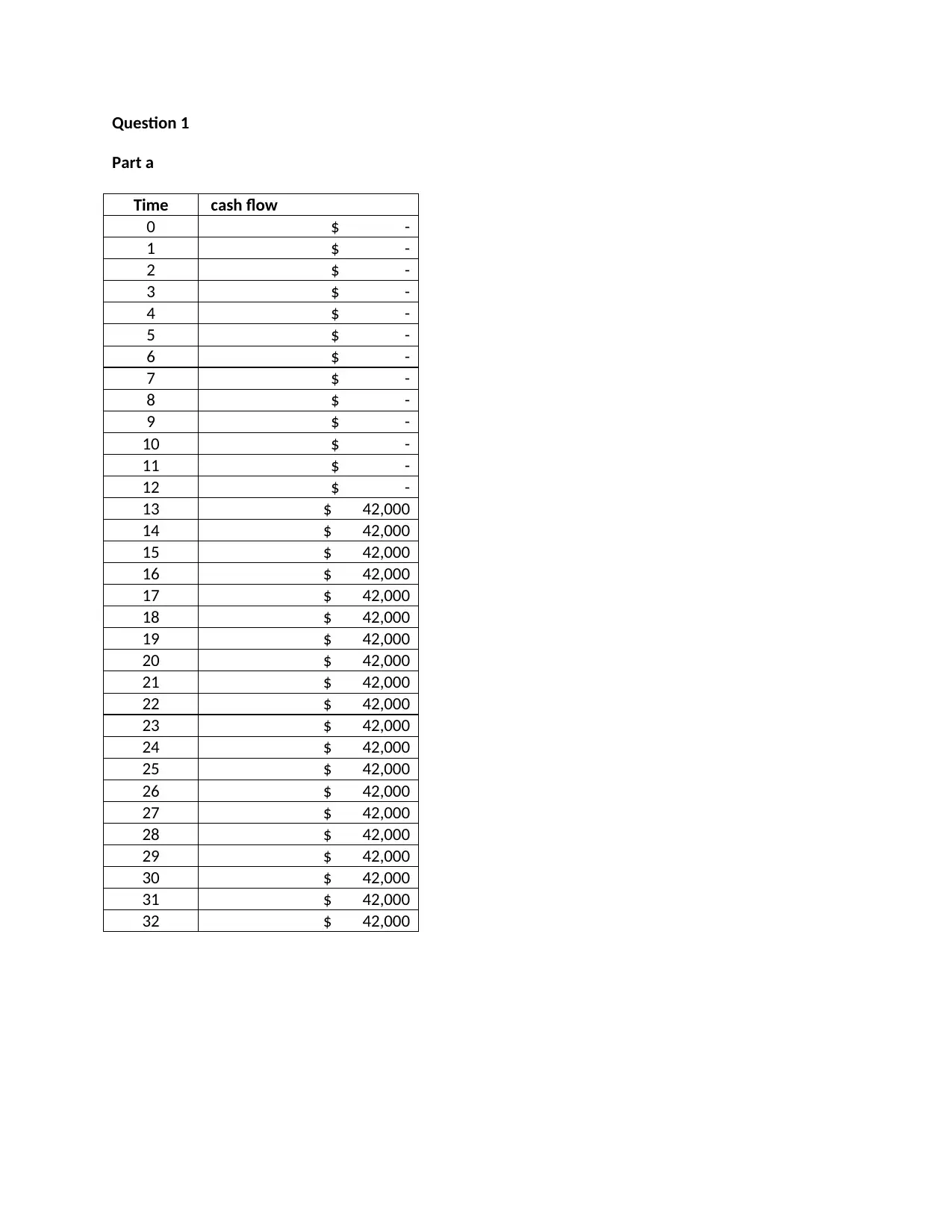
Question 1
Part a
Time cash flow
0 $ -
1 $ -
2 $ -
3 $ -
4 $ -
5 $ -
6 $ -
7 $ -
8 $ -
9 $ -
10 $ -
11 $ -
12 $ -
13 $ 42,000
14 $ 42,000
15 $ 42,000
16 $ 42,000
17 $ 42,000
18 $ 42,000
19 $ 42,000
20 $ 42,000
21 $ 42,000
22 $ 42,000
23 $ 42,000
24 $ 42,000
25 $ 42,000
26 $ 42,000
27 $ 42,000
28 $ 42,000
29 $ 42,000
30 $ 42,000
31 $ 42,000
32 $ 42,000

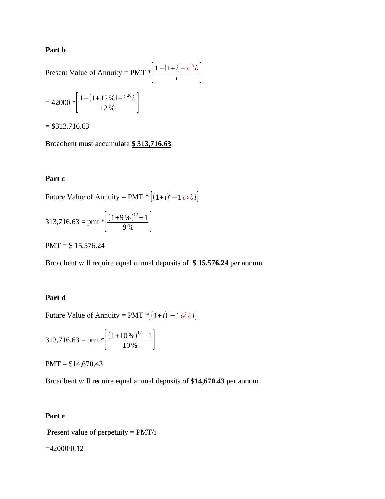
Part b
Present Value of Annuity = PMT * [ 1− ( 1+ i ) −¿15 ¿
i ]
= 42000 * [ 1− ( 1+12% ) −¿20 ¿
12 % ]
= $313,716.63
Broadbent must accumulate $ 313,716.63
Part c
Future Value of Annuity = PMT * [ (1+ i)n−1 ¿¿¿ i ]
313,716.63 = pmt * [ (1+9 %)12−1
9 % ]
PMT = $ 15,576.24
Broadbent will require equal annual deposits of $ 15,576.24 per annum
Part d
Future Value of Annuity = PMT * [ (1+i)n−1 ¿¿¿ i ]
313,716.63 = pmt * [ (1+10 %)12−1
10 % ]
PMT = $14,670.43
Broadbent will require equal annual deposits of $14,670.43 per annum
Part e
Present value of perpetuity = PMT/i
=42000/0.12

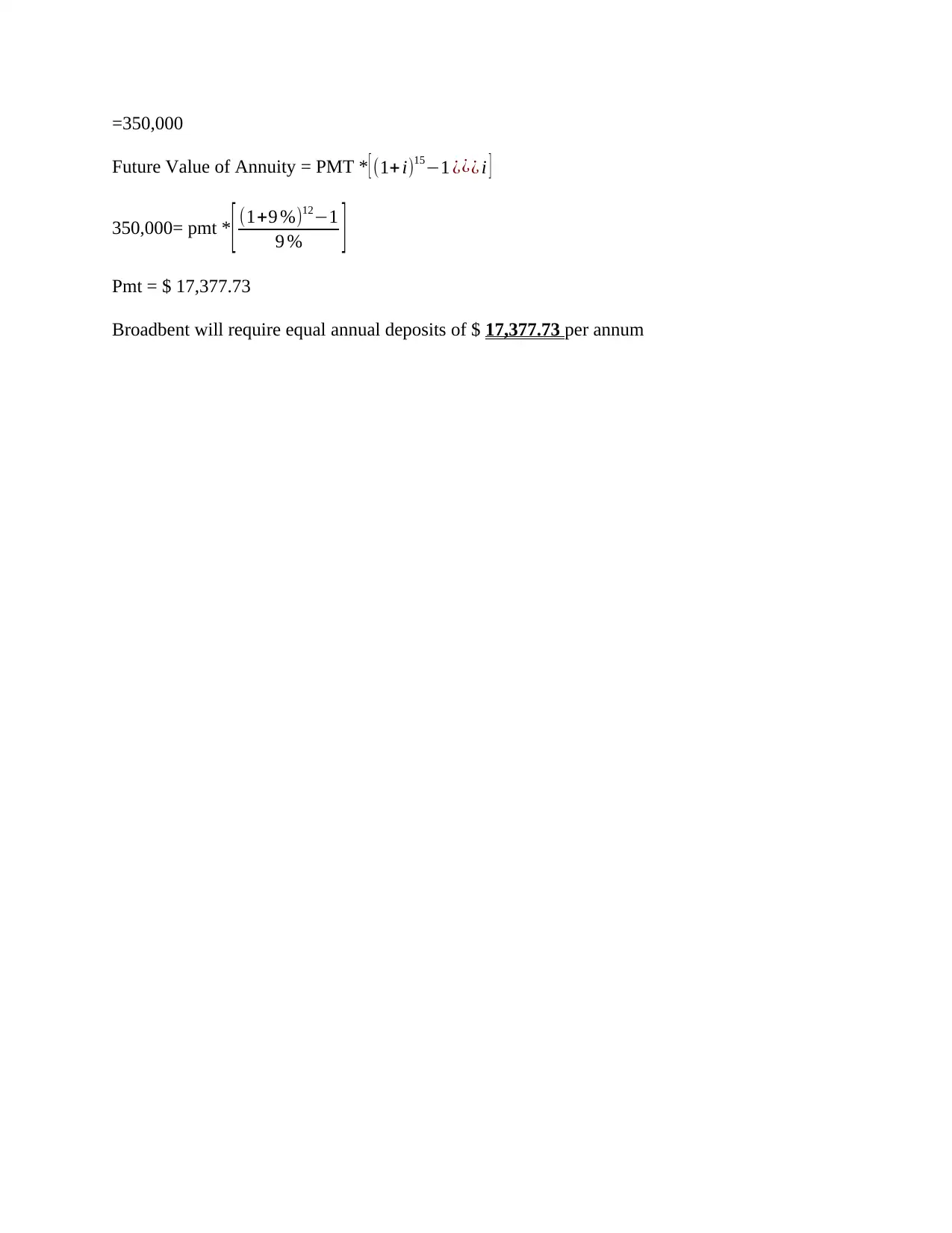
=350,000
Future Value of Annuity = PMT * [ (1+i)15−1 ¿¿¿ i ]
350,000= pmt * [ (1+9 %)12−1
9 % ]
Pmt = $ 17,377.73
Broadbent will require equal annual deposits of $ 17,377.73 per annum

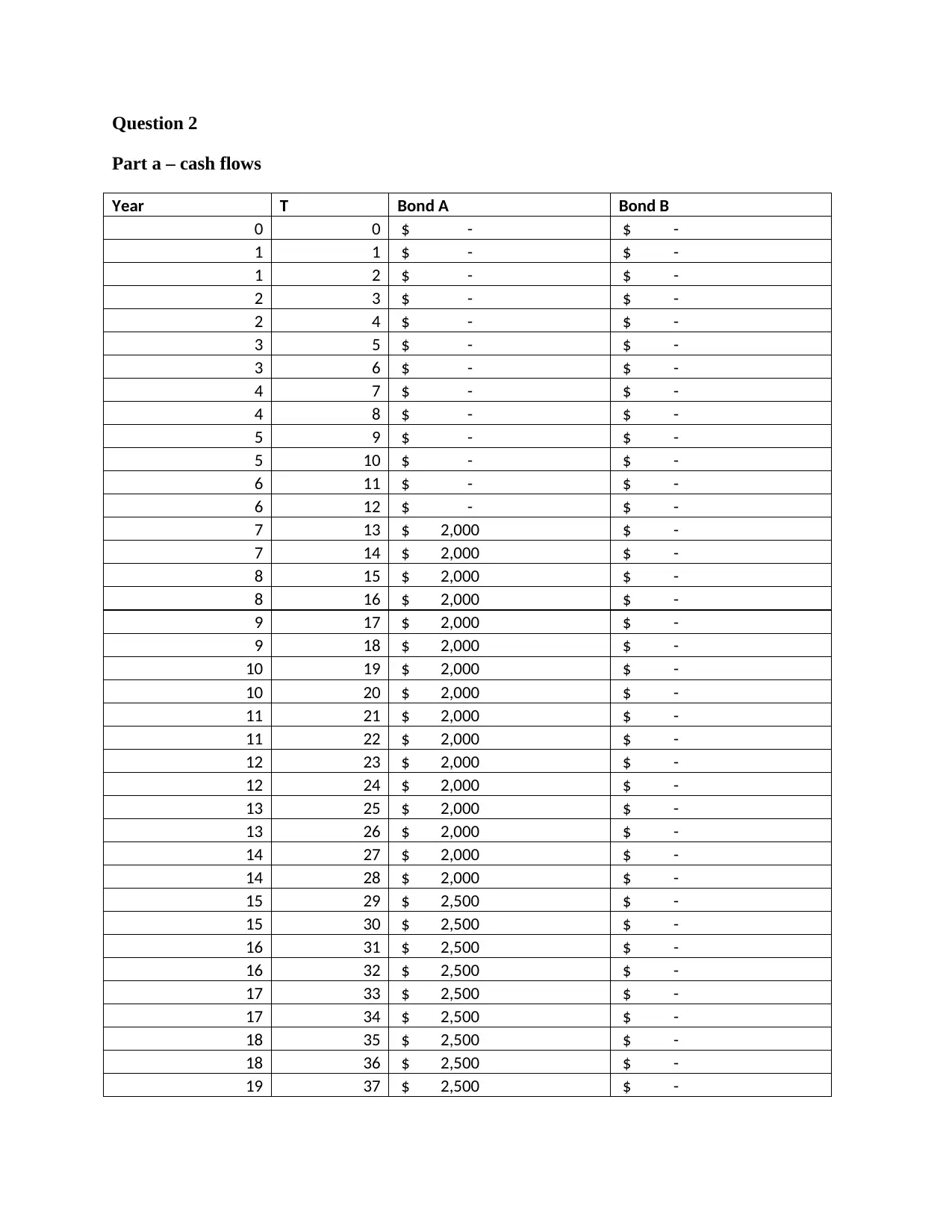
Question 2
Part a – cash flows
Year T Bond A Bond B
0 0 $ - $ -
1 1 $ - $ -
1 2 $ - $ -
2 3 $ - $ -
2 4 $ - $ -
3 5 $ - $ -
3 6 $ - $ -
4 7 $ - $ -
4 8 $ - $ -
5 9 $ - $ -
5 10 $ - $ -
6 11 $ - $ -
6 12 $ - $ -
7 13 $ 2,000 $ -
7 14 $ 2,000 $ -
8 15 $ 2,000 $ -
8 16 $ 2,000 $ -
9 17 $ 2,000 $ -
9 18 $ 2,000 $ -
10 19 $ 2,000 $ -
10 20 $ 2,000 $ -
11 21 $ 2,000 $ -
11 22 $ 2,000 $ -
12 23 $ 2,000 $ -
12 24 $ 2,000 $ -
13 25 $ 2,000 $ -
13 26 $ 2,000 $ -
14 27 $ 2,000 $ -
14 28 $ 2,000 $ -
15 29 $ 2,500 $ -
15 30 $ 2,500 $ -
16 31 $ 2,500 $ -
16 32 $ 2,500 $ -
17 33 $ 2,500 $ -
17 34 $ 2,500 $ -
18 35 $ 2,500 $ -
18 36 $ 2,500 $ -
19 37 $ 2,500 $ -

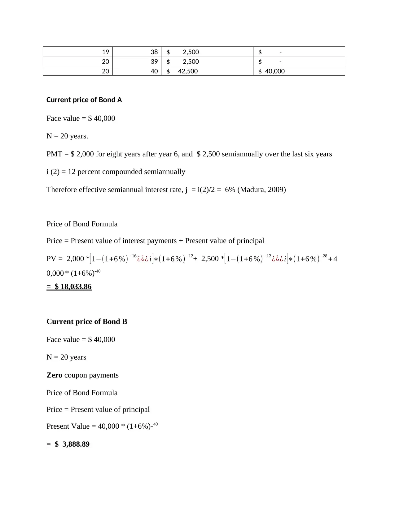
19 38 $ 2,500 $ -
20 39 $ 2,500 $ -
20 40 $ 42,500 $ 40,000
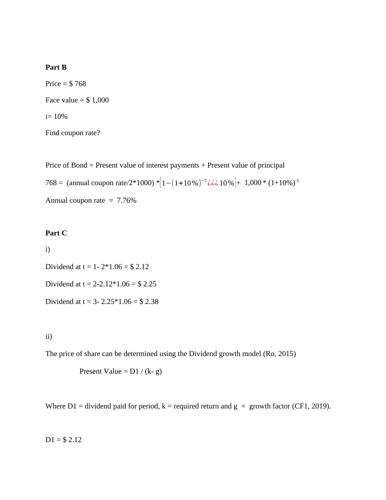
Current price of Bond A
Face value = $ 40,000
N = 20 years.
PMT = $ 2,000 for eight years after year 6, and $ 2,500 semiannually over the last six years
i (2) = 12 percent compounded semiannually
Therefore effective semiannual interest rate, j = i(2)/2 = 6% (Madura, 2009)
Price of Bond Formula
Price = Present value of interest payments + Present value of principal
PV = 2,000 *[ 1−(1+6 %)−16 ¿¿¿ i ]∗(1+6 % )−12+ 2,500 *[ 1−(1+6 %)−12 ¿¿¿ i ]∗(1+6 %)−28 + 4
0,000 * (1+6%)-40
= $ 18,033.86
Current price of Bond B
Face value = $ 40,000
N = 20 years
Zero coupon payments
Price of Bond Formula
Price = Present value of principal
Present Value = 40,000 * (1+6%)-40
= $ 3,888.89

Part B
Price = $ 768
Face value = $ 1,000
i= 10%
Find coupon rate?
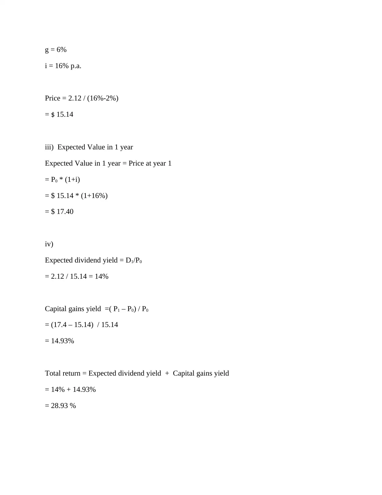
Price of Bond = Present value of interest payments + Present value of principal
768 = (annual coupon rate/2*1000) *[ 1−(1+10 %)−5 ¿¿¿ 10 % ]+ 1,000 * (1+10%)-5
Annual coupon rate = 7.76%
Part C
i)
Dividend at t = 1- 2*1.06 = $ 2.12
Dividend at t = 2-2.12*1.06 = $ 2.25
Dividend at t = 3- 2.25*1.06 = $ 2.38
ii)
The price of share can be determined using the Dividend growth model (Ro, 2015)
Present Value = D1 / (k- g)
Where D1 = dividend paid for period, k = required return and g = growth factor (CF1, 2019).
D1 = $ 2.12

g = 6%
i = 16% p.a.
Price = 2.12 / (16%-2%)
= $ 15.14
iii) Expected Value in 1 year
Expected Value in 1 year = Price at year 1
= P0 * (1+i)
= $ 15.14 * (1+16%)
= $ 17.40
iv)
Expected dividend yield = D1/P0
= 2.12 / 15.14 = 14%
Capital gains yield =( P1 – P0) / P0
= (17.4 – 15.14) / 15.14
= 14.93%
Total return = Expected dividend yield + Capital gains yield
= 14% + 14.93%
= 28.93 %

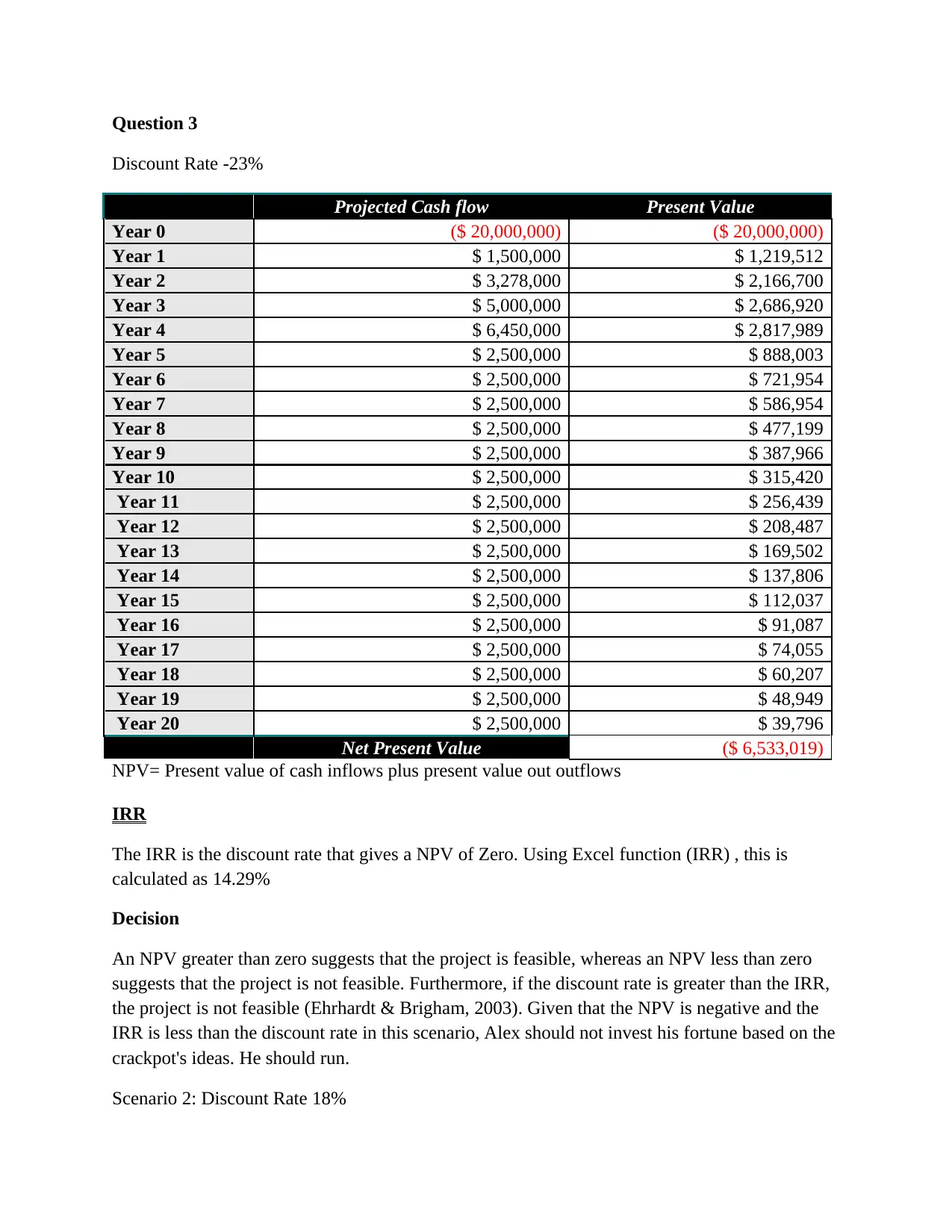
Question 3
Discount Rate -23%
Projected Cash flow Present Value
Year 0 ($ 20,000,000) ($ 20,000,000)
Year 1 $ 1,500,000 $ 1,219,512
Year 2 $ 3,278,000 $ 2,166,700
Year 3 $ 5,000,000 $ 2,686,920
Year 4 $ 6,450,000 $ 2,817,989
Year 5 $ 2,500,000 $ 888,003
Year 6 $ 2,500,000 $ 721,954
Year 7 $ 2,500,000 $ 586,954
Year 8 $ 2,500,000 $ 477,199
Year 9 $ 2,500,000 $ 387,966
Year 10 $ 2,500,000 $ 315,420
Year 11 $ 2,500,000 $ 256,439
Year 12 $ 2,500,000 $ 208,487
Year 13 $ 2,500,000 $ 169,502
Year 14 $ 2,500,000 $ 137,806
Year 15 $ 2,500,000 $ 112,037
Year 16 $ 2,500,000 $ 91,087
Year 17 $ 2,500,000 $ 74,055
Year 18 $ 2,500,000 $ 60,207
Year 19 $ 2,500,000 $ 48,949
Year 20 $ 2,500,000 $ 39,796
Net Present Value ($ 6,533,019)
NPV= Present value of cash inflows plus present value out outflows
IRR
The IRR is the discount rate that gives a NPV of Zero. Using Excel function (IRR) , this is
calculated as 14.29%
Decision
An NPV greater than zero suggests that the project is feasible, whereas an NPV less than zero
suggests that the project is not feasible. Furthermore, if the discount rate is greater than the IRR,
the project is not feasible (Ehrhardt & Brigham, 2003). Given that the NPV is negative and the
IRR is less than the discount rate in this scenario, Alex should not invest his fortune based on the
crackpot's ideas. He should run.
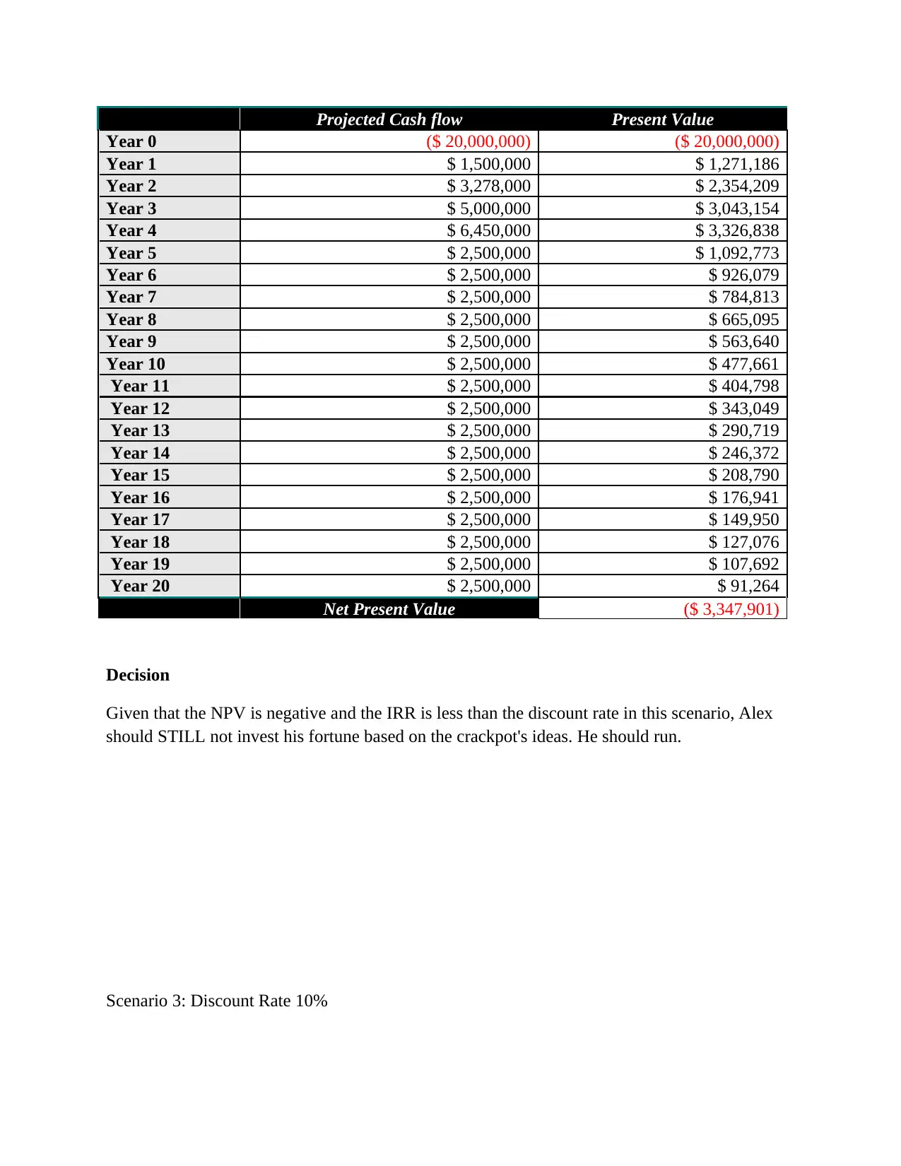
Scenario 2: Discount Rate 18%

Projected Cash flow Present Value
Year 0 ($ 20,000,000) ($ 20,000,000)
Year 1 $ 1,500,000 $ 1,271,186
Year 2 $ 3,278,000 $ 2,354,209
Year 3 $ 5,000,000 $ 3,043,154
Year 4 $ 6,450,000 $ 3,326,838
Year 5 $ 2,500,000 $ 1,092,773
Year 6 $ 2,500,000 $ 926,079
Year 7 $ 2,500,000 $ 784,813
Year 8 $ 2,500,000 $ 665,095
Year 9 $ 2,500,000 $ 563,640
Year 10 $ 2,500,000 $ 477,661
Year 11 $ 2,500,000 $ 404,798
Year 12 $ 2,500,000 $ 343,049
Year 13 $ 2,500,000 $ 290,719
Year 14 $ 2,500,000 $ 246,372
Year 15 $ 2,500,000 $ 208,790
Year 16 $ 2,500,000 $ 176,941
Year 17 $ 2,500,000 $ 149,950
Year 18 $ 2,500,000 $ 127,076
Year 19 $ 2,500,000 $ 107,692
Year 20 $ 2,500,000 $ 91,264
Net Present Value ($ 3,347,901)
Decision
Given that the NPV is negative and the IRR is less than the discount rate in this scenario, Alex
should STILL not invest his fortune based on the crackpot's ideas. He should run.
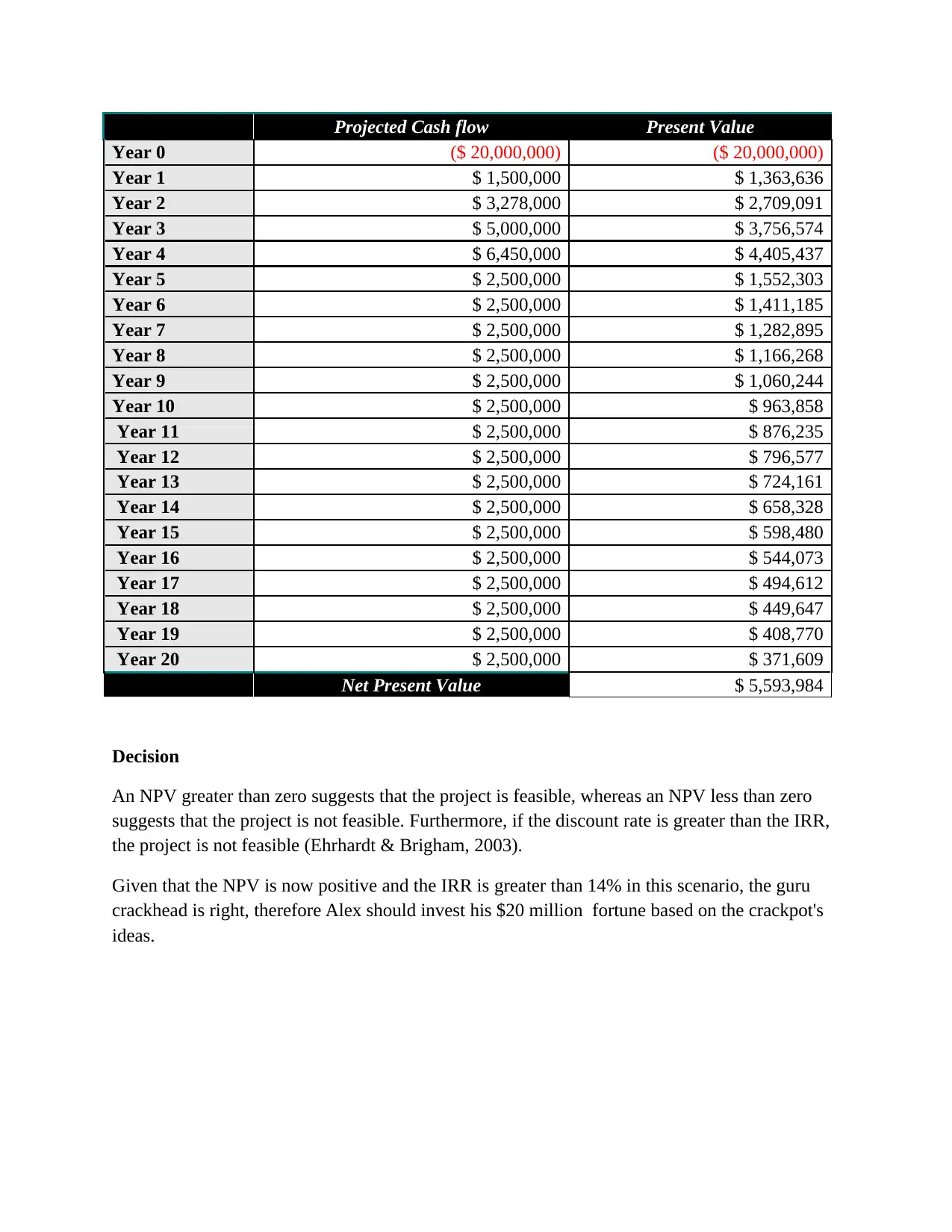
Scenario 3: Discount Rate 10%

Projected Cash flow Present Value
Year 0 ($ 20,000,000) ($ 20,000,000)
Year 1 $ 1,500,000 $ 1,363,636
Year 2 $ 3,278,000 $ 2,709,091
Year 3 $ 5,000,000 $ 3,756,574
Year 4 $ 6,450,000 $ 4,405,437
Year 5 $ 2,500,000 $ 1,552,303
Year 6 $ 2,500,000 $ 1,411,185
Year 7 $ 2,500,000 $ 1,282,895
Year 8 $ 2,500,000 $ 1,166,268
Year 9 $ 2,500,000 $ 1,060,244
Year 10 $ 2,500,000 $ 963,858
Year 11 $ 2,500,000 $ 876,235
Year 12 $ 2,500,000 $ 796,577
Year 13 $ 2,500,000 $ 724,161
Year 14 $ 2,500,000 $ 658,328
Year 15 $ 2,500,000 $ 598,480
Year 16 $ 2,500,000 $ 544,073
Year 17 $ 2,500,000 $ 494,612
Year 18 $ 2,500,000 $ 449,647
Year 19 $ 2,500,000 $ 408,770
Year 20 $ 2,500,000 $ 371,609
Net Present Value $ 5,593,984
Decision
An NPV greater than zero suggests that the project is feasible, whereas an NPV less than zero
suggests that the project is not feasible. Furthermore, if the discount rate is greater than the IRR,
the project is not feasible (Ehrhardt & Brigham, 2003).
Given that the NPV is now positive and the IRR is greater than 14% in this scenario, the guru
crackhead is right, therefore Alex should invest his $20 million fortune based on the crackpot's
ideas.

Question 4
Part A
DREXLA OGATO
Weight 20% 80%
PRICE $ 6.00 $ 4.00
Re 18% 14%
Σ 22% 20%
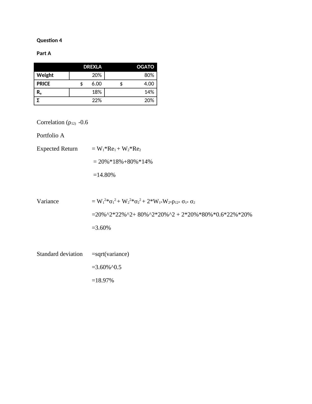
Correlation (ρ12) -0.6
Portfolio A
Expected Return = W1*Re1 + W2*Re2
= 20%*18%+80%*14%
=14.80%
Variance = W12*σ12 + W22*σ22 + 2*W1*W2*ρ12* σ1* σ2
=20%^2*22%^2+ 80%^2*20%^2 + 2*20%*80%*0.6*22%*20%
=3.60%
Standard deviation =sqrt(variance)
=3.60%^0.5
=18.97%

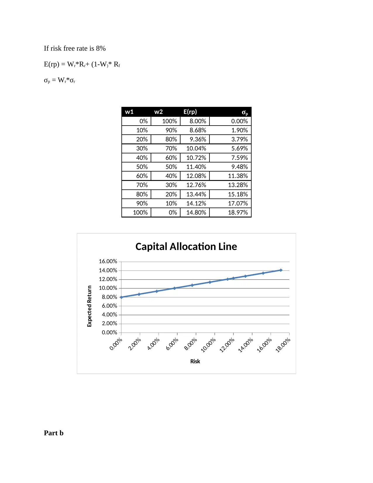
If risk free rate is 8%
E(rp) = Wr*Rr+ (1-W)* Rf
σp = Wr*σr
w1 w2 E(rp) σp
0% 100% 8.00% 0.00%
10% 90% 8.68% 1.90%
20% 80% 9.36% 3.79%
30% 70% 10.04% 5.69%
40% 60% 10.72% 7.59%
50% 50% 11.40% 9.48%
60% 40% 12.08% 11.38%
70% 30% 12.76% 13.28%
80% 20% 13.44% 15.18%
90% 10% 14.12% 17.07%
100% 0% 14.80% 18.97%
0.00%
2.00%
4.00%
6.00%
8.00%
10.00%
12.00%
14.00%
16.00%
18.00%
0.00%
2.00%
4.00%
6.00%
8.00%
10.00%
12.00%
14.00%
16.00%
Capital Allocation Line
Risk
Expected Return
Part b