Deakin University: Real World Analytics - Energy Efficiency Analysis

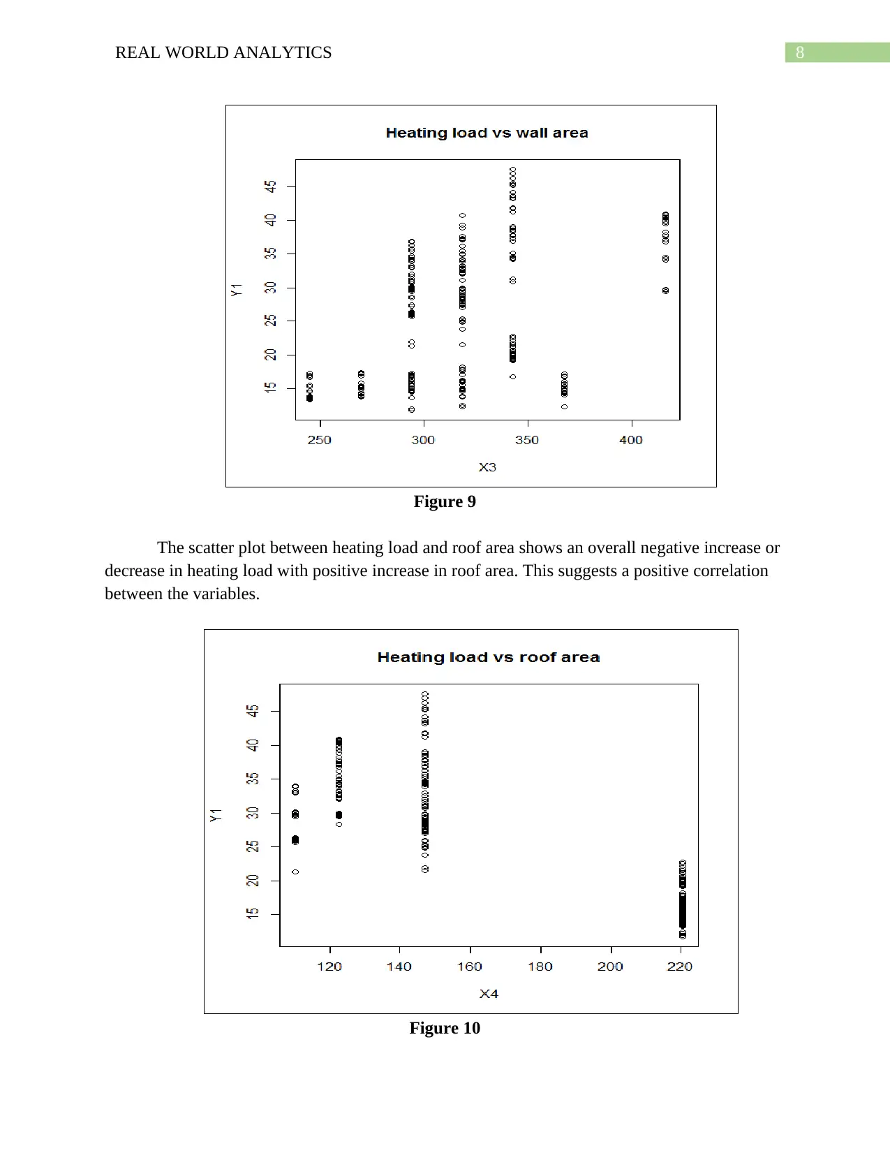
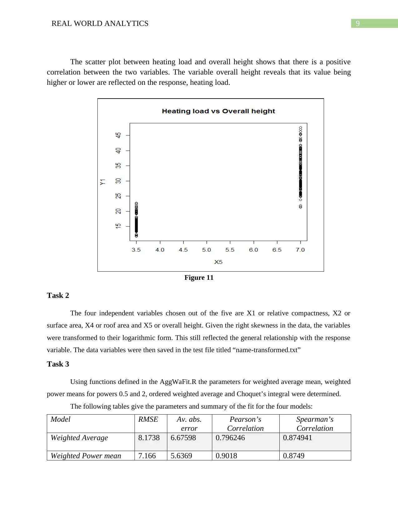
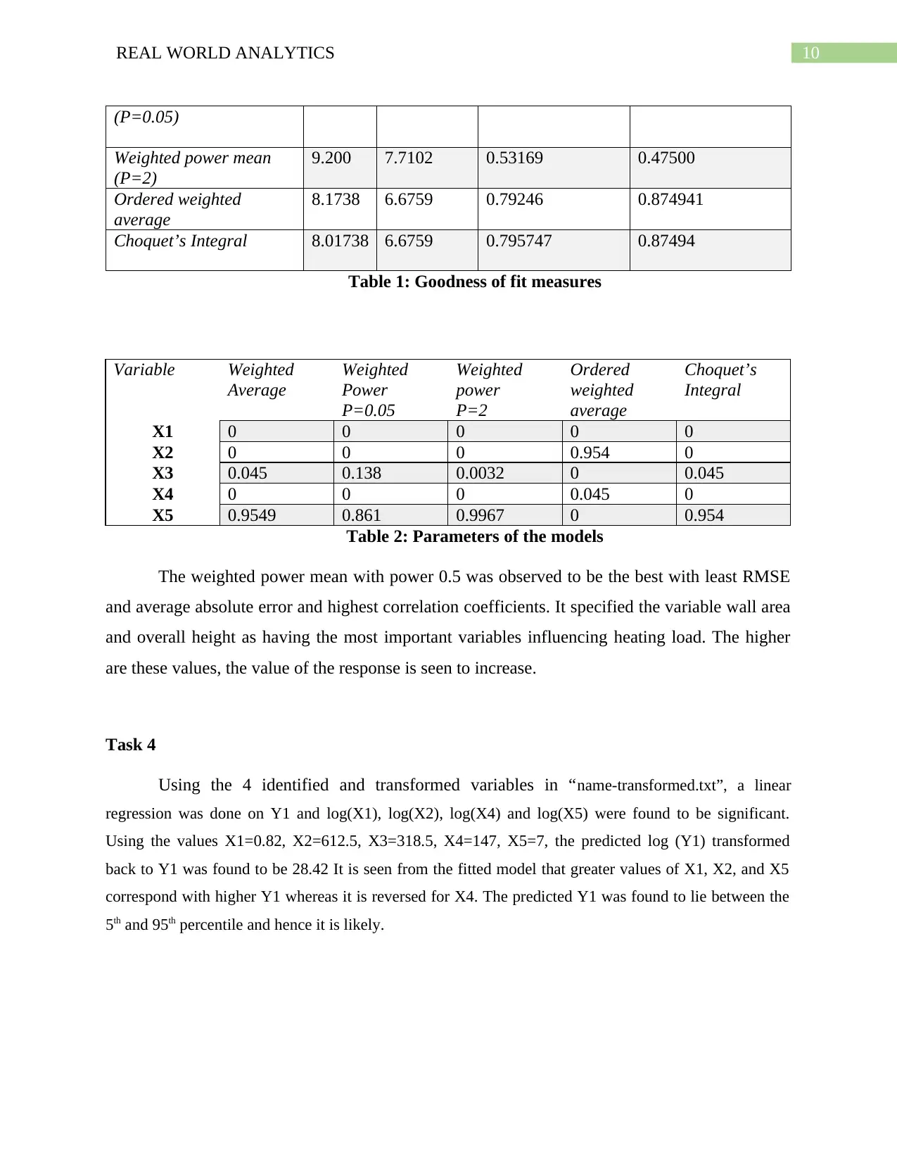
This project analyzes an energy efficiency dataset for buildings, focusing on heating and cooling loads. The analysis, conducted in R, involves examining variables such as relative compactness, surface area, wall area, roof area, and overall height. Task 1 includes data loading, graphical summarization, and exploration of relationships between variables. Task 2 involves data transformation and saving the data. Task 3 uses the AggWaFit.R functions to determine parameters for various models, including weighted average mean, weighted power means, ordered weighted average, and Choquet’s integral, and compares their goodness of fit. Task 4 performs linear regression on transformed variables and predicts heating load. Part B involves a juice mixture optimization problem using linear programming to minimize cost, considering constraints related to ingredient proportions and demand.

Running head: REAL WORLD ANALYTICS
REAL WORLD ANALYTICS
Name of Student
Name of University

1REAL WORLD ANALYTICS
Table of Contents
Part A: Analysis of Energy Efficiency Dataset for Buildings.........................................................2
Description...................................................................................................................................2
Task 1...........................................................................................................................................2
Task 2...........................................................................................................................................9
Task 3...........................................................................................................................................9
Task 4.........................................................................................................................................10
Part B.............................................................................................................................................11
1.................................................................................................................................................11

2REAL WORLD ANALYTICS
Part A: Analysis of Energy Efficiency Dataset for Buildings
Description
Heating load and cooling load are important determinants of the specifications in the
heating and cooling equipment used in designing efficient buildings. Therefore tools for energy
simulation to predict energy consumption of a building is necessary to anticipate these
parameters and hence design structures which can accommodate the demand optimally, keeping
in line with the idea of energy efficient buildings.
The variables Heating load (HL or denoted by Y1) and cooling load (CL or Y2) are made the
two suggested variables of interest for this paper and the variables, relative compactness in
percentage or X1, Surface area in square meters or X2, wall area in square meters or X3, roof
area in square meters or X4 and overall height in meters or X5 are taken as potential
predictors of the chosen response, heating load. 768 building data units were simulated through a
building simulator and the data on the above mentioned variables were noted and hence used for
the analysis. The analysis was done in R.
Task 1
The text data file ENB18data.txt was downloaded from CloudDeakin and into the R
working directory. The data was hence loaded into the R console and assigned to a data matrix,
namely, “the.data”. The matrix consisted of 7 columns to accommodate each variable and 786
rows of simulated data observations.
The response variable Heating Load or Y1 was chosen as the variable of interest and it’s
the influence of the variables denoted by X1, X2, X3, X4 and X5 was analyzed and each of the
variables were individually scrutinized as well. The analysis was done on the basis of a sample
of size 300 chosen by use of simple random sampling process in R.
The graphical summarization of each variable and the relationship between the response
variable and each individual independent variables are depicted and discussed hence.The
histogram of the response variable depicts that heating load in KWh per meter square per annum
follows a right skewed distribution that is most of its values seem to be concentrated towards the
lower or left tail making its right tail more elongated than its left. The mode is indicated to lie in
the interval 15KWh per meter square to 20KWh per meter square.

3REAL WORLD ANALYTICS
Figure 1
The relative compactness values are seen to be more or less evenly distributed around
center lying between 0.6 and 1.
Figure 2

4REAL WORLD ANALYTICS
The surface area is seen to be more or less evenly and symmetrically distributed around
the center with a slight skewness towards right. The values range from 500 to 850 with the modal
class being the interval 600 to 650.
Figure 3
The wall area are seen to vary between the values 200 and 500 and the values are
seen to be distributed is a right skewed shape with modal class in the interval 290 to 300 meter
squared.
Figure 4

5REAL WORLD ANALYTICS
The histogram of the roof area suggests a discrete distribution with distinct disjointed
bins with at least four distinct values of roof area present in the data. It is suggested that roof
areas thus have limited number of specifications which are abided by in the market and thus or
otherwise reflected in the simulated data. The values lie between 110 and 230 meter squared.
Figure 5
Two distinct bins is made apparent from the histogram of overall height one between 3.5
and 4 and the other between 6.5 and 7. The data is suggested as being discrete and thus it is
indicated that overall height are maintained to be either a value between 6.5 and 7 or 3.5 and 4.

6REAL WORLD ANALYTICS
Figure 6
Next, the relationship between each independent variable and the variable of interest is
considered. It is observed that heating load tends to be more for higher values of compactness.
The highest heating load is observed to be between compactness values between 0.75 and 0.8.

7REAL WORLD ANALYTICS
Figure 7
The heating load is seen to be lower for greater surface area. Thus a negative correlation
is suggested between heating load and surface area.
Figure 8
The variation in heating load does not seem to be much linearly affected by that of the
wall area. The pattern of heating load does not seem to be clearly increasing or decreasing with
changes in the wall area.

8REAL WORLD ANALYTICS
Figure 9
The scatter plot between heating load and roof area shows an overall negative increase or
decrease in heating load with positive increase in roof area. This suggests a positive correlation
between the variables.
Figure 10

9REAL WORLD ANALYTICS
The scatter plot between heating load and overall height shows that there is a positive
correlation between the two variables. The variable overall height reveals that its value being
higher or lower are reflected on the response, heating load.
Figure 11
Task 2
The four independent variables chosen out of the five are X1 or relative compactness, X2 or
surface area, X4 or roof area and X5 or overall height. Given the right skewness in the data, the variables
were transformed to their logarithmic form. This still reflected the general relationship with the response
variable. The data variables were then saved in the test file titled “name-transformed.txt”
Task 3
Using functions defined in the AggWaFit.R the parameters for weighted average mean, weighted
power means for powers 0.5 and 2, ordered weighted average and Choquet’s integral were determined.
The following tables give the parameters and summary of the fit for the four models:
Model RMSE Av. abs.
error
Pearson’s
Correlation
Spearman’s
Correlation
Weighted Average 8.1738 6.67598 0.796246 0.874941
Weighted Power mean 7.166 5.6369 0.9018 0.8749

10REAL WORLD ANALYTICS
(P=0.05)
Weighted power mean
(P=2)
9.200 7.7102 0.53169 0.47500
Ordered weighted
average
8.1738 6.6759 0.79246 0.874941
Choquet’s Integral 8.01738 6.6759 0.795747 0.87494
Table 1: Goodness of fit measures
Variable Weighted
Average
Weighted
Power
P=0.05
Weighted
power
P=2
Ordered
weighted
average
Choquet’s
Integral
X1 0 0 0 0 0
X2 0 0 0 0.954 0
X3 0.045 0.138 0.0032 0 0.045
X4 0 0 0 0.045 0
X5 0.9549 0.861 0.9967 0 0.954
Table 2: Parameters of the models
The weighted power mean with power 0.5 was observed to be the best with least RMSE
and average absolute error and highest correlation coefficients. It specified the variable wall area
and overall height as having the most important variables influencing heating load. The higher
are these values, the value of the response is seen to increase.
Task 4
Using the 4 identified and transformed variables in “name-transformed.txt”, a linear
regression was done on Y1 and log(X1), log(X2), log(X4) and log(X5) were found to be significant.
Using the values X1=0.82, X2=612.5, X3=318.5, X4=147, X5=7, the predicted log (Y1) transformed
back to Y1 was found to be 28.42 It is seen from the fitted model that greater values of X1, X2, and X5
correspond with higher Y1 whereas it is reversed for X4. The predicted Y1 was found to lie between the
5th and 95th percentile and hence it is likely.

11REAL WORLD ANALYTICS
Part B
1.
a)
A special juice is to be made out of two juices JA and JB. Cost of juice JA is set to be $6 and cost
of juice JB is $5. Let X1 be the amount of juice JA and X2 be the amount of juice JB. The special juice is
to be made up of at the least 3.5 litres Orange per 100 litres, 4 litres Apple concentrate per 100 litres and
at most 6 litres Carrot concentrate. Again then it was directed that at least 50 litres of the special juice was
in demand per week.
Hence the list of constraints are:
 6X1+3X2>=3.5
 3X1+6X2>=4
 4X1+8X2<=6
 X1+X2>=50
Furthermore the amount of JA and JB obviously cannot be less than 0. Thus there also exists two
additional non negativity constraints, X1>=0 and X2>=0.
The amount of juice X1 and X2 to be used in the mixture is to be determined such that the cost of
making the special juice is minimized. Therefore the problem at hand is a minimization problem. The cost
function is: 6X1 + 5X2 where coefficient of X1 is price of JA per litres and coefficient of X2 is the same
for JB. Hence given the aforementioned constraints the cost function ought to be minimized.