Building and Evaluating Predictive Models: BUS5PA Assignment 1 (2017)

This assignment report details a predictive analytics project (BUS5PA) undertaken at La Trobe Business School in 2017. The project focuses on building and evaluating predictive models using SAS software. The student explores exploratory data analysis, decision tree modeling, and regression-based modeling. The analysis includes data partitioning, model selection based on average square error and misclassification rate, and model comparison to determine the best performing model. The project compares decision tree models and regression models to predict customer behavior, specifically the purchase of organic products. The report also discusses the strengths and weaknesses of each modeling approach and concludes with a discussion on data mining techniques and their applications.

Building and Evaluating Predictive Models
Assignment 1
(BUS5PA Predictive Analytics – Semester 2, 2017)
By
<Student Name>
(19152818)
La Trobe Business School
Australia

Table of Contents
1. Setting up the project and exploratory analysis 4
2. Decision tree based modeling and analysis 5
3. Regression based modeling and analysis 7
4. Open ended discussion 8
5. Extending current knowledge with additional reading 12
References 14
Annexure A
1

List of Figures
Figure 1 Project: BUS5PA_Assignment1_ 19152818....................................................................A
Figure 2 New Library.....................................................................................................................A
Figure 3 New data source: Organics...............................................................................................A
Figure 4 Column Metadata.............................................................................................................B
Figure 5 Organics purchase indicator (%age).................................................................................B
Figure 6 Organics diagram workspace: Organics data source........................................................C
Figure 7 Data partition....................................................................................................................C
Figure 8 Data set Allocations..........................................................................................................C
Figure 9 Addition of Decision Tree................................................................................................C
Figure 10 Autonomously created decision tree model...................................................................D
Figure 11 Assessment measure.......................................................................................................D
Figure 12 Subtree Assessment Plot................................................................................................D
Figure 13 Decision Tree (Tree 1)....................................................................................................E
Figure 14 Decision Tree after adding Tree 2..................................................................................E
Figure 15 Three-way Split...............................................................................................................F
Figure 16 Assessment Measure : Decision Tree 2..........................................................................F
2

Figure 17 Average square error : Tree 2.........................................................................................F
Figure 18 StatExplore tool..............................................................................................................G
Figure 19 Default input method updation.......................................................................................G
Figure 20 Indicator variables..........................................................................................................G
Figure 21 Addition of Regression model........................................................................................H
Figure 22 Regression Model Selection...........................................................................................H
Figure 23 Result of Regression model.............................................................................................I
Figure 24 Summary of Stepwise Selection......................................................................................I
Figure 25 Odd ratio Estimates..........................................................................................................J
Figure 26 Average squared error (ASE)..........................................................................................J
Figure 27 Model Comparison.........................................................................................................K
Figure 28 Model Comparison Result..............................................................................................K
Figure 29 ROC Chart......................................................................................................................L
Figure 30 Cumulative Lift...............................................................................................................L
Figure 31 Fit Statistics...................................................................................................................M
List of Tables
Table 1 Model performance comparison 8
3

1. Setting up the project and exploratory analysis
a] New project named BUS5PA_Assignment1_19152818 has been created, which has been
shown in Figure 1.
a.1] New SAS library named has been created named As52818, and data source has been
created using SAS dataset ORGANICS, which has been mentioned above in Figure 2 and
Figure 3.
a.2] As mentioned in the business case assignment, all the roles have been set, Figure 4 shows
the roles which have been defined for the data source ORGANICS.
a.3] “TargetBuy” has been defined as target variable. 24.77% individuals have purchased
organic products and rest i.e. 75.23% have not purchased organic products, which has been
depicted in Figure 5.
a.4] As mentioned in Figure 4, Demcluster has been set rejected.
a.5] Data source named organics has been defined, which has been shown in Figure 3
a.6] ORGANICS data source has been added to Organics diagram workspace, which has been
shown in Figure 6.
b] TargetAmt cannot be used as an input for a model that is used to predict TargetBuy,
TargetBuy indicates if the individuals have purchased the organic item or not, whereas
TargetAmt indicates the number of organic amounts bought. TargetAmt will only be
4

recorded for those who have purchased any organic products i.e. when Targetbuy is Yes.
Hence, TargetAmt can never be the predictor of TargetBuy. In this business case as an initial
buyer incentive plan, the supermarket’s objective is to develop loyalty model by whether
customers have purchased any of the organic products. So, TargetBuy is the perfectly
suitable as target variable
2. Decision tree based modeling and analysis
a] Data partition node has been added to the diagram from Sample Tab, and it has been
connected to the data source node i.e. ORGANICS. 50% of the data have been assigned in
training and rest 50% have been added in validation, which has been depicted in Figure 7 and
Figure 8.
b] Decision Tree node has been added to the workspace and it has been connected to the Data
partition node, which has been depicted in Figure 9.
c] Decision Tree has been built autonomously, not interactively, and sub tree model assessment
criteria has been chosen as Use average square error which has been shown in Figure 10 and
11.
c.1] As per average square error, there are 29 leaves in the optimal tree, subtree assessment plot
has been shown in Figure 12.
c.2] Age has been used for the first split, it has partitioned the training data in two parts, first
subset was for the age less than 44.5, for this subset TargetBuy = 1 has higher than average
5

concentration. Second subset is for age greater than or equals to 44.5, for the second subset
TargetBuy = 0 has higher than average concentration. Autonomously created decision tree
model, using average square error assessment, has been depicted in Figure 13.
d] Second Decision Tree has been added to the diagram, and it has been connected to the Data
Partition node (shown in Figure 14).
d.1] The maximum number of branch has been set 3 to allow three-way splits, shown in Figure
15.
d.2] Creation of decision tree model using average square error has been shown in Figure 16.
d.3] As per average square error, there are 33 leaves in the optimal tree, subtree assessment plot
has been shown in Figure 17. In C, there were 29 leaves in the optimal tree. With the
decision tree, Tree 2, misclassification rate (Train:0.1848) of the model is very marginally
lower than the model with the decision tree, Tree 1 (Train: 0.1851) and average square error
of the model with the decision tree, Tree 1 (Train: 0.1329) is lower than the model with the
decision tree, Tree 2 (Train: 0.1330). Hence it can be said that tree with 29 leaves performs
marginally better in terms of average square error and tree with 33 leaves performs
marginally better in terms of misclassification rate. But with the higher number of leaves
complexity increases, a less complex and reliable tree may be appropriate.
e] Average square error evaluates the tree which has the smallest average square error among
the actual class and predicted class, based on the average square error decision tree model
with Tree 1 appears better than model with Tree 2, as Average square error (Tree 1 Model) <
6

Average square error (Tree 2 Model) i.e. 0.1329 < 0.1330. lower average squared error
indicates the model performs better as a predictor because it is “wrong” less often.
3. Regression based modeling and analysis
a] From the explorer tab of Toolbar, StatExplore tool has been added to the ORGANICS data
source and run that, which has been shown in Figure 18.
b] In preparation for regression, missing value imputation is needed, as in SAS Miner
regressions models ignore observations which contain missing values, that usually reduces
the size of the training data. Less training data can considerably weaken the predictive power
of these models. In this case, we will use the imputation to overcome the hindrance of
missing data, impute missing values before fit the models are required. It is also necessary to
impute missing values before fitting a model that overlooks observations with missing values
while comparing those models with a decision tree.
c] For class variables, Default Input Method has been set to Default Constant Value and Default
Character Value has been set to U, and for interval variables Default Input Method is Mean
(shown in Figure 19). To create imputation indicators for all imputed inputs, Indicator
Variable Type has been set as Unique, and Indicator Variable Role has been set to Input
(shown in Figure 20).
d] Regression node has been added to the diagram and connected to the Impute node (shown in
Figure 21).
7

e] Selection Model has been set as Stepwise, and Selection Criteria has been set to Validation
Error, which has been depicted in Figure 22.
f] Result of the regression model has been shown in Figure 23. The selected model, based on
the error rate for the validation data, is the model trained in Step 6. Which consists of the
following variables: IMP_DemAffl, IMP_DemAge, IMP_DemGender, M_DemAffl,
M_DemAge and M_DemGender (i.e. Affluence grade, Age and Gender) (Figure 24). Hence,
for the supermarket management Affluence grade, age and gender would be main parameters
to understand loyalty of consumers and to formulate a predictive model. The result of odds
ratio estimates shows that important parameter for this model will be imputed value of
gender (Female), gender (Male), Affluence grade and age. The average squared error (ASE)
of prediction is used to estimate the error in prediction of a model fitted using the training
data shown below in Equation 1 (Atkinson, 1980)
ASE= 1
n ∑ ( yi− ^yi )2…………………………………………Equation 1
Here yi is the ith observation in the validation data set and ^yi is its predicted value using the
fitted model and n is the validation sample size. The ASE output SAS has been shown in
Figure 26. ASE for this model is 0.138587 (train data) and 0.137156 (validation data). In a
modeling context, a good predictive model produces values that are close to these ASE
values. An overfit model produces a smaller ASE on the training data but higher values on the
validation and test data. An underfit model exhibits higher values for all data roles.
8

4. Open ended discussion
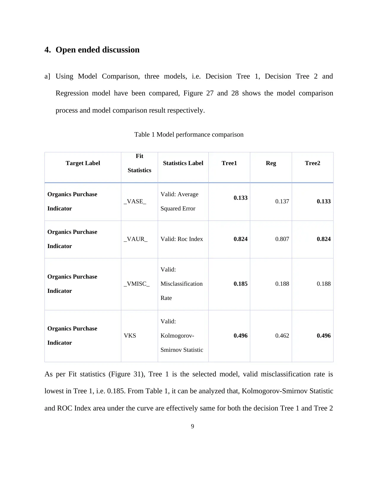
a] Using Model Comparison, three models, i.e. Decision Tree 1, Decision Tree 2 and
Regression model have been compared, Figure 27 and 28 shows the model comparison
process and model comparison result respectively.
Table 1 Model performance comparison
Target Label
Fit
Statistics
Statistics Label Tree1 Reg Tree2
Organics Purchase
Indicator
_VASE_
Valid: Average
Squared Error
0.133 0.137 0.133
Organics Purchase
Indicator
_VAUR_ Valid: Roc Index 0.824 0.807 0.824
Organics Purchase
Indicator
_VMISC_
Valid:
Misclassification
Rate
0.185 0.188 0.188
Organics Purchase
Indicator
VKS
Valid:
Kolmogorov-
Smirnov Statistic
0.496 0.462 0.496
As per Fit statistics (Figure 31), Tree 1 is the selected model, valid misclassification rate is
lowest in Tree 1, i.e. 0.185. From Table 1, it can be analyzed that, Kolmogorov-Smirnov Statistic
and ROC Index area under the curve are effectively same for both the decision Tree 1 and Tree 2
9

model, and perform slightly better than regression model. For average squared error are also
effectively same for Tree 1 and Tree 2, and performs better than Regression model. Hence, it can
be concluded that Tree 1 is better performer than other two models.
b] The data mining can be defined as a collection of various methods. For a unique business case,
an individual preparation and method selection is required. There is no strict instruction on
which method should be implemented in a situation. as mentioned in the previous section, in
this business case, after analyzing the three models, decision tree 1 is the best performer.
The decision tree induction is a method mainly based on two principles. The first principle is
called divide rule. This indicates, that in every step, the data would be split into two or more
parts and the algorithm continues recursively on individual parts (Máša & Kočka, 1996). The
second principle is called the greedy principle, which indicates that the splitting is based only on
limited information. Decision trees are mainly used for predictions, classifications and
descriptions. The decision tree is a classifier with a very high capacity. But, in real scenarios,
decision trees may tend to overfitting. The logistic regression (Berry & Linoff, 1997; Rud, 2001)
is a method which originated from the statistics, but it is often used in data mining applications.
The main objective of this method is to predict (to classify) a binary (categorical) variable
(Dreiseitl & Ohno-Machado, 2002). The logistic regression has smaller capacity than decision
trees. In real Scenarios, the risk of overfitting is not that high, but the logistic regression is not
able to fit some distributions.
So, it can be said that,
10

 Both the methods are efficient
 Logistic regression will perform better if there's a single decision boundary, but not
necessarily parallel to the axis (Friedman, Hastie, & Tibshirani, 2000).
 Decision trees can be implemented to situations where there's not just one underlying
decision boundary, but many, and will perform best if the class labels roughly lie in
hyper-rectangular regions.
 Logistic regression is intrinsically simple, it has low variance and so is less prone to over-
fitting. Decision trees can be scaled up to be very complex, are more accountable to over-
fit. Pruning can be applied to avoid this.
Hence, decision trees are also frequently used in pre-processing phase for a logistic
regression. Decision trees with a logistic regression is one of the major techniques used for
prediction and classification.
c] Decision Trees are advantageous for predictive modeling due to:
 Implicit variable screening and selection – the top nodes of the tree are the most important
variables in the dataset! (Swain & Hauska, 1977)
 Less data preparation– data does not need to be normalized, and decision trees are less
sensitive to missing data and outliers (Rokach & Maimon, 2014)
 Decision trees do not require assumptions of linearity
 Decision tree output is graphical and easy to explain i.e. decision based on cut points
11