BUQU 1230 Extra Assignment 1: Statistical Analysis, Spring 2020
VerifiedAdded on 2022/09/07
|11
|1839
|12
Homework Assignment
AI Summary
This document presents the solutions to BUQU 1230 Extra Assignment 1, focusing on statistical concepts and their applications. The assignment covers a range of topics, including point estimation, confidence intervals, and sample size calculations related to a bicycle helmet law observation. It then delves into sampling distributions, calculating the standard error and probabilities related to rainfall during kayaking trips. Finally, the assignment addresses hypothesis testing, requiring the formulation of null and alternative hypotheses, calculation of point estimates, p-values, and interpretation of results to determine if there is a significant difference in tipping behavior between California and British Columbia. The solutions are comprehensive and include detailed explanations, formulas, and interpretations of the statistical findings.
Extra Assignment # 1 / Spring, 2020
BUQU 1230 – Extra Assignment #1 (In Partial Replacement of Midterm & Final Exam)
Instructions:
1. Type your answers into this document. Save your work and upload it back to the course
Moodle website. Please keep in mind I won’t see your Excel work, so document all the
work you want me to see in this file.
2. You are both encouraged and permitted to use Excel to the utmost of your ability for this
assignment. This is an open textbook / open Internet assignment. You may find the
formula sheet on our Moodle website especially useful.
3. This assignment is due on Tuesday, March 31, 2020.
Question 1 ___ out of 11
Question 2 ___ out of 5
Question 3 ___ out of 10
Total ___ out of 26
Paraphrase This Document
Need a fresh take? Get an instant paraphrase of this document with our AI Paraphraser
Extra Assignment # 1 / Spring, 2020
Solutions
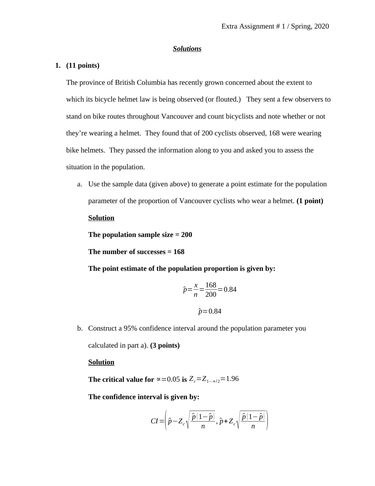
1. (11 points)
The province of British Columbia has recently grown concerned about the extent to
which its bicycle helmet law is being observed (or flouted.) They sent a few observers to
stand on bike routes throughout Vancouver and count bicyclists and note whether or not
they’re wearing a helmet. They found that of 200 cyclists observed, 168 were wearing
bike helmets. They passed the information along to you and asked you to assess the
situation in the population.
a. Use the sample data (given above) to generate a point estimate for the population
parameter of the proportion of Vancouver cyclists who wear a helmet. (1 point)
Solution
The population sample size = 200
The number of successes = 168
The point estimate of the population proportion is given by:
^p= x
n =168
200 =0.84
^p=0.84
b. Construct a 95% confidence interval around the population parameter you
calculated in part a). (3 points)
Solution
The critical value for ∝=0.05 is Zc=Z1−∝/ 2=1.96
The confidence interval is given by:
CI =( ^p−Zc √ ^p ( 1− ^p )
n , ^p+ Zc √ ^p ( 1− ^p )
n )
Solutions
1. (11 points)
The province of British Columbia has recently grown concerned about the extent to
which its bicycle helmet law is being observed (or flouted.) They sent a few observers to
stand on bike routes throughout Vancouver and count bicyclists and note whether or not
they’re wearing a helmet. They found that of 200 cyclists observed, 168 were wearing
bike helmets. They passed the information along to you and asked you to assess the
situation in the population.
a. Use the sample data (given above) to generate a point estimate for the population
parameter of the proportion of Vancouver cyclists who wear a helmet. (1 point)
Solution
The population sample size = 200
The number of successes = 168
The point estimate of the population proportion is given by:
^p= x
n =168
200 =0.84
^p=0.84
b. Construct a 95% confidence interval around the population parameter you
calculated in part a). (3 points)
Solution
The critical value for ∝=0.05 is Zc=Z1−∝/ 2=1.96
The confidence interval is given by:
CI =( ^p−Zc √ ^p ( 1− ^p )
n , ^p+ Zc √ ^p ( 1− ^p )
n )
Extra Assignment # 1 / Spring, 2020
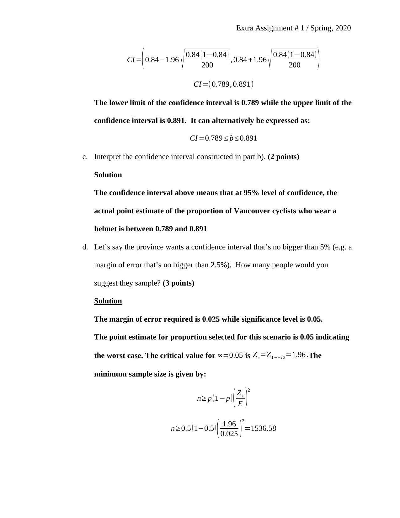
CI =( 0.84−1.96 √ 0.84 ( 1−0.84 )
200 , 0.84 +1.96 √ 0.84 ( 1−0.84 )
200 )
CI =( 0.789, 0.891)
The lower limit of the confidence interval is 0.789 while the upper limit of the
confidence interval is 0.891. It can alternatively be expressed as:
CI =0.789 ≤ ^p ≤ 0.891
c. Interpret the confidence interval constructed in part b). (2 points)
Solution
The confidence interval above means that at 95% level of confidence, the
actual point estimate of the proportion of Vancouver cyclists who wear a
helmet is between 0.789 and 0.891
d. Let’s say the province wants a confidence interval that’s no bigger than 5% (e.g. a
margin of error that’s no bigger than 2.5%). How many people would you
suggest they sample? (3 points)
Solution
The margin of error required is 0.025 while significance level is 0.05.
The point estimate for proportion selected for this scenario is 0.05 indicating
the worst case. The critical value for ∝=0.05 is Zc=Z1−∝/ 2=1.96 .The
minimum sample size is given by:
n ≥ p ( 1−p ) ( Zc
E )2
n ≥ 0.5 ( 1−0.5 ) ( 1.96
0.025 )2
=1536.58
⊘ This is a preview!⊘
Do you want full access?
Subscribe today to unlock all pages.
Trusted by 1+ million students worldwide
Extra Assignment # 1 / Spring, 2020
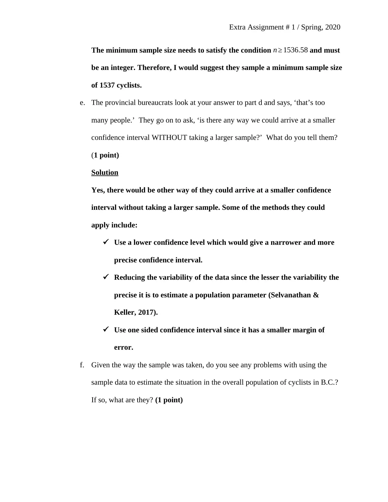
The minimum sample size needs to satisfy the condition n ≥ 1536.58 and must
be an integer. Therefore, I would suggest they sample a minimum sample size
of 1537 cyclists.
e. The provincial bureaucrats look at your answer to part d and says, ‘that’s too
many people.’ They go on to ask, ‘is there any way we could arrive at a smaller
confidence interval WITHOUT taking a larger sample?’ What do you tell them?
(1 point)
Solution
Yes, there would be other way of they could arrive at a smaller confidence
interval without taking a larger sample. Some of the methods they could
apply include:
Use a lower confidence level which would give a narrower and more
precise confidence interval.
Reducing the variability of the data since the lesser the variability the
precise it is to estimate a population parameter (Selvanathan &
Keller, 2017).
Use one sided confidence interval since it has a smaller margin of
error.
f. Given the way the sample was taken, do you see any problems with using the
sample data to estimate the situation in the overall population of cyclists in B.C.?
If so, what are they? (1 point)
Paraphrase This Document
Need a fresh take? Get an instant paraphrase of this document with our AI Paraphraser
Extra Assignment # 1 / Spring, 2020
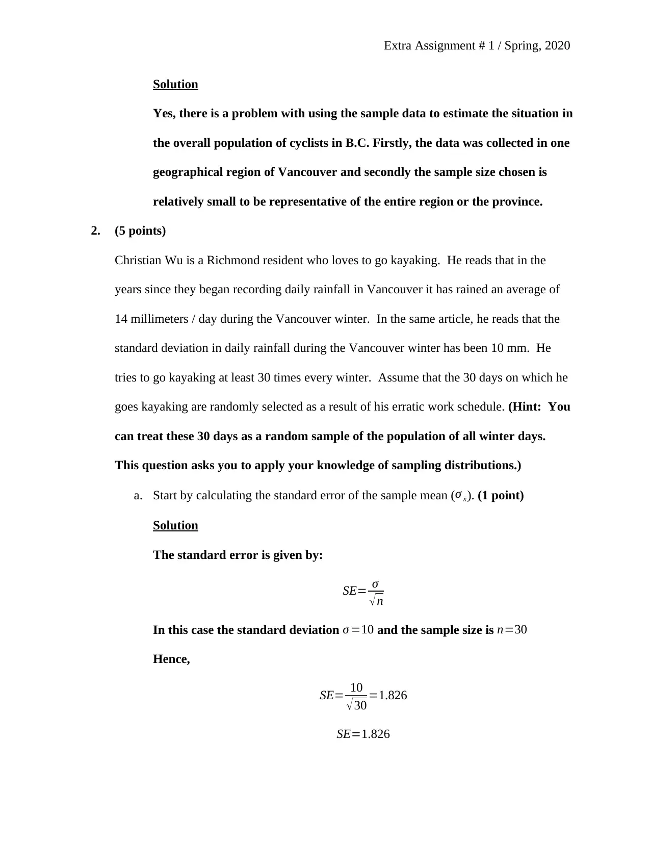
Solution
Yes, there is a problem with using the sample data to estimate the situation in
the overall population of cyclists in B.C. Firstly, the data was collected in one
geographical region of Vancouver and secondly the sample size chosen is
relatively small to be representative of the entire region or the province.
2. (5 points)
Christian Wu is a Richmond resident who loves to go kayaking. He reads that in the
years since they began recording daily rainfall in Vancouver it has rained an average of
14 millimeters / day during the Vancouver winter. In the same article, he reads that the
standard deviation in daily rainfall during the Vancouver winter has been 10 mm. He
tries to go kayaking at least 30 times every winter. Assume that the 30 days on which he
goes kayaking are randomly selected as a result of his erratic work schedule. (Hint: You
can treat these 30 days as a random sample of the population of all winter days.
This question asks you to apply your knowledge of sampling distributions.)
a. Start by calculating the standard error of the sample mean (σ x). (1 point)
Solution
The standard error is given by:
SE= σ
√ n
In this case the standard deviation σ =10 and the sample size is n=30
Hence,
SE= 10
√30 =1.826
SE=1.826
Solution
Yes, there is a problem with using the sample data to estimate the situation in
the overall population of cyclists in B.C. Firstly, the data was collected in one
geographical region of Vancouver and secondly the sample size chosen is
relatively small to be representative of the entire region or the province.
2. (5 points)
Christian Wu is a Richmond resident who loves to go kayaking. He reads that in the
years since they began recording daily rainfall in Vancouver it has rained an average of
14 millimeters / day during the Vancouver winter. In the same article, he reads that the
standard deviation in daily rainfall during the Vancouver winter has been 10 mm. He
tries to go kayaking at least 30 times every winter. Assume that the 30 days on which he
goes kayaking are randomly selected as a result of his erratic work schedule. (Hint: You
can treat these 30 days as a random sample of the population of all winter days.
This question asks you to apply your knowledge of sampling distributions.)
a. Start by calculating the standard error of the sample mean (σ x). (1 point)
Solution
The standard error is given by:
SE= σ
√ n
In this case the standard deviation σ =10 and the sample size is n=30
Hence,
SE= 10
√30 =1.826
SE=1.826
Extra Assignment # 1 / Spring, 2020
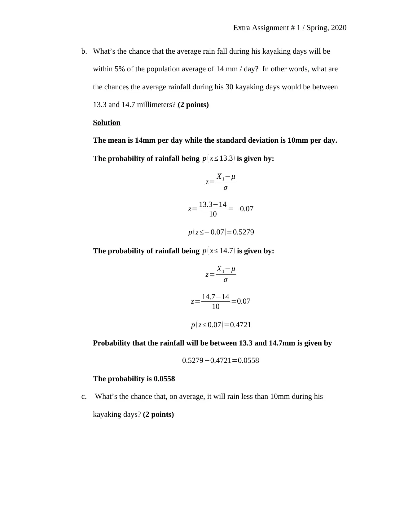
b. What’s the chance that the average rain fall during his kayaking days will be
within 5% of the population average of 14 mm / day? In other words, what are
the chances the average rainfall during his 30 kayaking days would be between
13.3 and 14.7 millimeters? (2 points)
Solution
The mean is 14mm per day while the standard deviation is 10mm per day.
The probability of rainfall being p ( x ≤ 13.3 ) is given by:
z= X1−μ
σ
z= 13.3−14
10 =−0.07
p ( z ≤−0.07 )=0.5279
The probability of rainfall being p ( x ≤ 14.7 ) is given by:
z= X1−μ
σ
z= 14.7−14
10 =0.07
p ( z ≤ 0.07 ) =0.4721
Probability that the rainfall will be between 13.3 and 14.7mm is given by
0.5279−0.4721=0.0558
The probability is 0.0558
c. What’s the chance that, on average, it will rain less than 10mm during his
kayaking days? (2 points)
⊘ This is a preview!⊘
Do you want full access?
Subscribe today to unlock all pages.
Trusted by 1+ million students worldwide
Extra Assignment # 1 / Spring, 2020
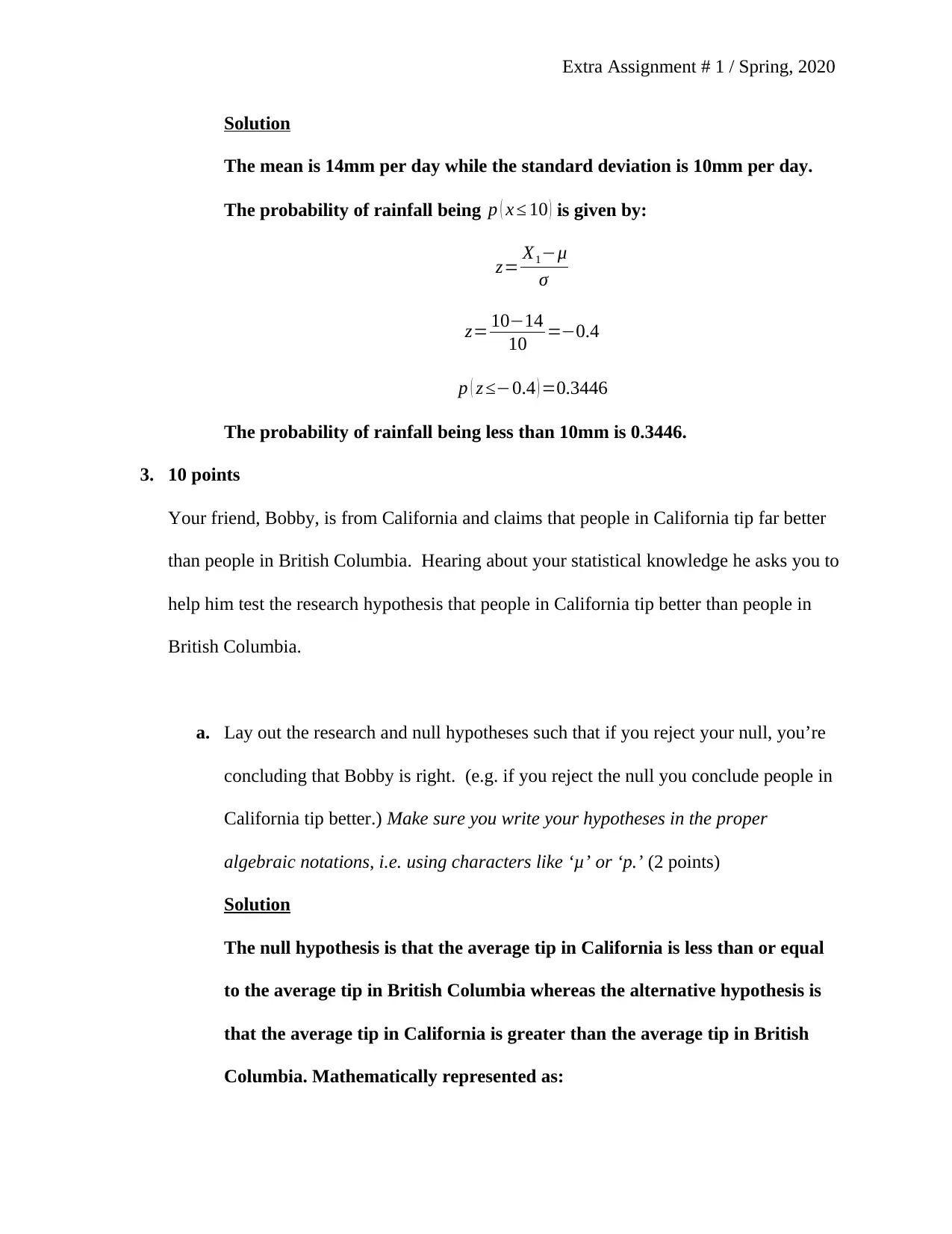
Solution
The mean is 14mm per day while the standard deviation is 10mm per day.
The probability of rainfall being p ( x ≤ 10 ) is given by:
z= X1−μ
σ
z= 10−14
10 =−0.4
p ( z ≤−0.4 ) =0.3446
The probability of rainfall being less than 10mm is 0.3446.
3. 10 points
Your friend, Bobby, is from California and claims that people in California tip far better
than people in British Columbia. Hearing about your statistical knowledge he asks you to
help him test the research hypothesis that people in California tip better than people in
British Columbia.
a. Lay out the research and null hypotheses such that if you reject your null, you’re
concluding that Bobby is right. (e.g. if you reject the null you conclude people in
California tip better.) Make sure you write your hypotheses in the proper
algebraic notations, i.e. using characters like ‘μ’ or ‘p.’ (2 points)
Solution
The null hypothesis is that the average tip in California is less than or equal
to the average tip in British Columbia whereas the alternative hypothesis is
that the average tip in California is greater than the average tip in British
Columbia. Mathematically represented as:
Solution
The mean is 14mm per day while the standard deviation is 10mm per day.
The probability of rainfall being p ( x ≤ 10 ) is given by:
z= X1−μ
σ
z= 10−14
10 =−0.4
p ( z ≤−0.4 ) =0.3446
The probability of rainfall being less than 10mm is 0.3446.
3. 10 points
Your friend, Bobby, is from California and claims that people in California tip far better
than people in British Columbia. Hearing about your statistical knowledge he asks you to
help him test the research hypothesis that people in California tip better than people in
British Columbia.
a. Lay out the research and null hypotheses such that if you reject your null, you’re
concluding that Bobby is right. (e.g. if you reject the null you conclude people in
California tip better.) Make sure you write your hypotheses in the proper
algebraic notations, i.e. using characters like ‘μ’ or ‘p.’ (2 points)
Solution
The null hypothesis is that the average tip in California is less than or equal
to the average tip in British Columbia whereas the alternative hypothesis is
that the average tip in California is greater than the average tip in British
Columbia. Mathematically represented as:
Paraphrase This Document
Need a fresh take? Get an instant paraphrase of this document with our AI Paraphraser
Extra Assignment # 1 / Spring, 2020
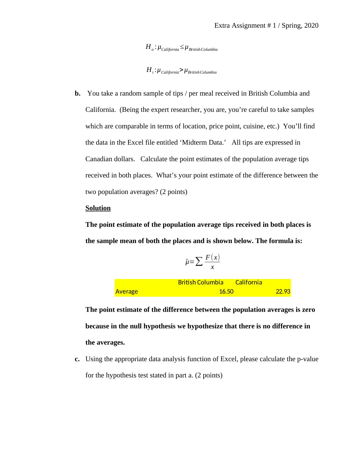
Ho : μCalifornia ≤ μBritishColumbia
Hi :μCalifornia > μBritish Columbia
b. You take a random sample of tips / per meal received in British Columbia and
California. (Being the expert researcher, you are, you’re careful to take samples
which are comparable in terms of location, price point, cuisine, etc.) You’ll find
the data in the Excel file entitled ‘Midterm Data.’ All tips are expressed in
Canadian dollars. Calculate the point estimates of the population average tips
received in both places. What’s your point estimate of the difference between the
two population averages? (2 points)
Solution
The point estimate of the population average tips received in both places is
the sample mean of both the places and is shown below. The formula is:
^μ=∑ F ( x)
x
British Columbia California
Average 16.50 22.93
The point estimate of the difference between the population averages is zero
because in the null hypothesis we hypothesize that there is no difference in
the averages.
c. Using the appropriate data analysis function of Excel, please calculate the p-value
for the hypothesis test stated in part a. (2 points)
Extra Assignment # 1 / Spring, 2020
Solution
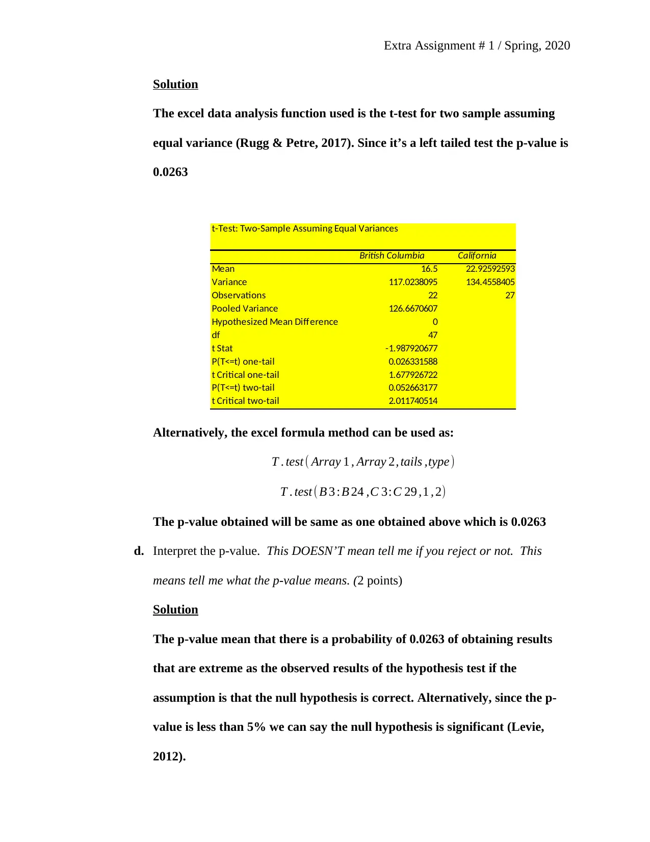
The excel data analysis function used is the t-test for two sample assuming
equal variance (Rugg & Petre, 2017). Since it’s a left tailed test the p-value is
0.0263
t-Test: Two-Sample Assuming Equal Variances
British Columbia California
Mean 16.5 22.92592593
Variance 117.0238095 134.4558405
Observations 22 27
Pooled Variance 126.6670607
Hypothesized Mean Difference 0
df 47
t Stat -1.987920677
P(T<=t) one-tail 0.026331588
t Critical one-tail 1.677926722
P(T<=t) two-tail 0.052663177
t Critical two-tail 2.011740514
Alternatively, the excel formula method can be used as:
T . test ( Array 1 , Array 2, tails ,type)
T . test (B 3 :B 24 ,C 3:C 29 ,1 , 2)
The p-value obtained will be same as one obtained above which is 0.0263
d. Interpret the p-value. This DOESN’T mean tell me if you reject or not. This
means tell me what the p-value means. (2 points)
Solution
The p-value mean that there is a probability of 0.0263 of obtaining results
that are extreme as the observed results of the hypothesis test if the
assumption is that the null hypothesis is correct. Alternatively, since the p-
value is less than 5% we can say the null hypothesis is significant (Levie,
2012).
Solution
The excel data analysis function used is the t-test for two sample assuming
equal variance (Rugg & Petre, 2017). Since it’s a left tailed test the p-value is
0.0263
t-Test: Two-Sample Assuming Equal Variances
British Columbia California
Mean 16.5 22.92592593
Variance 117.0238095 134.4558405
Observations 22 27
Pooled Variance 126.6670607
Hypothesized Mean Difference 0
df 47
t Stat -1.987920677
P(T<=t) one-tail 0.026331588
t Critical one-tail 1.677926722
P(T<=t) two-tail 0.052663177
t Critical two-tail 2.011740514
Alternatively, the excel formula method can be used as:
T . test ( Array 1 , Array 2, tails ,type)
T . test (B 3 :B 24 ,C 3:C 29 ,1 , 2)
The p-value obtained will be same as one obtained above which is 0.0263
d. Interpret the p-value. This DOESN’T mean tell me if you reject or not. This
means tell me what the p-value means. (2 points)
Solution
The p-value mean that there is a probability of 0.0263 of obtaining results
that are extreme as the observed results of the hypothesis test if the
assumption is that the null hypothesis is correct. Alternatively, since the p-
value is less than 5% we can say the null hypothesis is significant (Levie,
2012).
⊘ This is a preview!⊘
Do you want full access?
Subscribe today to unlock all pages.
Trusted by 1+ million students worldwide
Extra Assignment # 1 / Spring, 2020
e. Let’s say Bobby tells you he’s willing to accept 5% chance of being wrong.
What’s your conclusion? Do people in California appear to be better tippers than
people in British Columbia? (2 points)
Solution
The conclusion is that Bobby is not wrong since with 5% confidence level the
p-value is less than 0.05 indicating strong evidence against the null
hypothesis leading to its rejection in favor of alternative hypothesis (Shao,
2010). Its therefore true to say that people in California appear to be better
tippers than people British Columbia.
Paraphrase This Document
Need a fresh take? Get an instant paraphrase of this document with our AI Paraphraser
Extra Assignment # 1 / Spring, 2020
References
Levie, P.R. (2012). Advanced excel for scientific data analysis (2nd ed). New York, NY: Oxford
University Press.
Rugg, G., & Petre, M. (2017). A gentle guide to research methods. Maidenhead: Open
University Press.
Selvanathan, E. A., & Keller, G. (2017). Business statistics abridged (7th ed). South Melbourne,
Victoria: Cengage Learning.
Shao, J. (2010). Mathematical statistics (2nd ed). New York: Springer.
1 out of 11


Your All-in-One AI-Powered Toolkit for Academic Success.
+13062052269
info@desklib.com
Available 24*7 on WhatsApp / Email
![[object Object]](/_next/static/media/star-bottom.7253800d.svg)
Unlock your academic potential
Copyright © 2020–2026 A2Z Services. All Rights Reserved. Developed and managed by ZUCOL.