BUS102 Group Assignment: Production Possibility, Revenue, and Tax

This document provides a comprehensive solution to a BUS102 microeconomics group assignment. The assignment explores the concept of the production possibility frontier (PPF), analyzing its shape, properties, and implications for resource allocation. It further delves into revenue analysis, examining the relationship between price, quantity demanded, and revenue, including the concept of price elasticity of demand. The solution also addresses market equilibrium, consumer and producer surplus, and deadweight loss, using supply and demand diagrams to illustrate these concepts. Finally, the assignment analyzes the impact of a tax on alcohol, considering the inelastic nature of its demand, tax incidence, and the effectiveness of different policies to reduce consumption. The solution includes diagrams and references to support the analysis.

STUDENT NAME
COURSE NAME: BUS102 Group Assignment T217

A 1
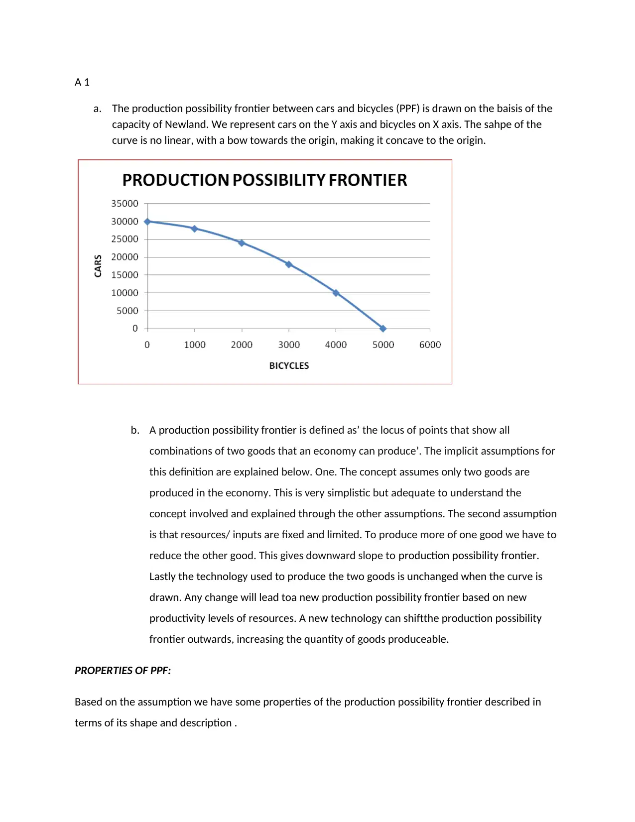
a. The production possibility frontier between cars and bicycles (PPF) is drawn on the baisis of the
capacity of Newland. We represent cars on the Y axis and bicycles on X axis. The sahpe of the
curve is no linear, with a bow towards the origin, making it concave to the origin.
b. A production possibility frontier is defined as’ the locus of points that show all
combinations of two goods that an economy can produce’. The implicit assumptions for
this definition are explained below. One. The concept assumes only two goods are
produced in the economy. This is very simplistic but adequate to understand the
concept involved and explained through the other assumptions. The second assumption
is that resources/ inputs are fixed and limited. To produce more of one good we have to
reduce the other good. This gives downward slope to production possibility frontier.
Lastly the technology used to produce the two goods is unchanged when the curve is
drawn. Any change will lead toa new production possibility frontier based on new
productivity levels of resources. A new technology can shiftthe production possibility
frontier outwards, increasing the quantity of goods produceable.
PROPERTIES OF PPF:
Based on the assumption we have some properties of the production possibility frontier described in
terms of its shape and description .

 DESCRIPTION OF ON PPC: we can understand the PPF through various points in the graph.
Any point that lies inside the curve implies unemployment of resources. Unused resources are
of no value and cause inefficiency, as idle resources do not contribute to economic value.
Any point that lies outside the curve is unattainable, while may be desirable. By the very
mathematical construction of the curve, such a point needs more resources, which are currently
unavailable.
Any point on the curve is EFFCICIENT, as all resources are used. To move between any two
points implies a reallocation of resources, while their full employment is intact.
 SHAPE: A production possibility frontier is bow shaped, due to the concept of opportunity costs
that are rising as we increase cars production. Opportunity cost of a car refers to the amount of
bicycles (alternative good) that must be given up to get 1 more bicycle produced. Cars have to
be given up as we have limited resources, with full employment of them. There is no other
option to increase bicycles without reducing cars. Increasing opportunity costs means that the
amount of cars we need to give up increases as bicycles rise. Assume we go from 1000 to 2000
bicycles, which requires a reduction of 4000 cars (=28000-24000). So opportunity cost of 1000
bicycles is 4000 cars.
Now let us go from 3000 to 4000 bicycles. This requires reduction of 8000 cars ( 18000-10000).
There has been a rise in cars that need to given up to gain the equal amount s of 1000 bicycles.
This demonstrates increasing opportunity costs concept. The cause is fully used resources which
are not equally efficient/productive at producing both cars and bicycles.
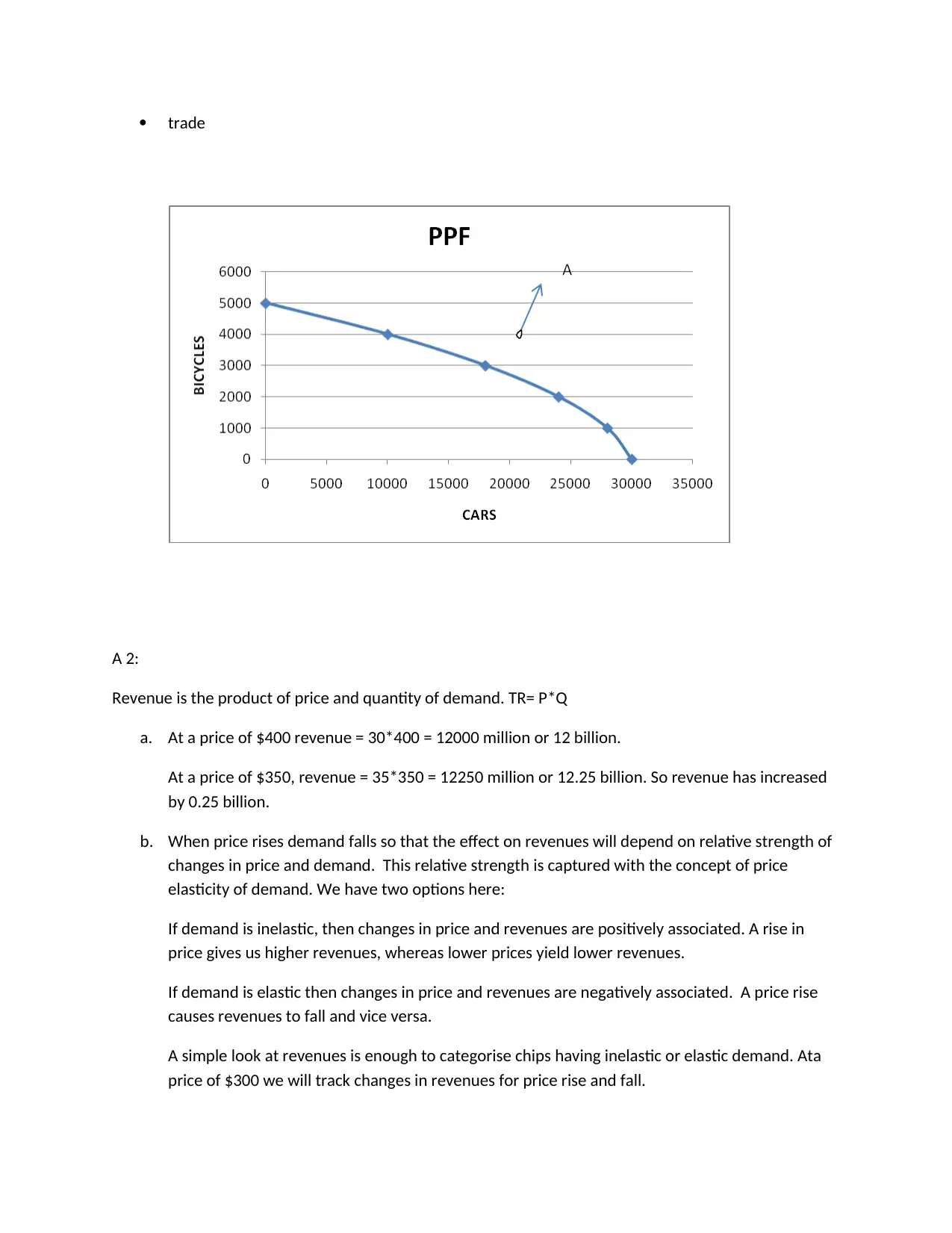
c. We start with production of 3000 bicycles and 18000 cars. We need to get 1000 more bicycles
and 2000 more cars. This means we need to increase both goods, which is impossible to do with
current resources and technology. This is because 3000 bicycles and 18000 cars we are already
on the PPF. As resources are limited we can’t increase both goods. To do so needs more
resources. We can reach A ( 4000 bicycles and 20000 cars), which does not lie on the PPC by
either one or a combination of the following, which will shift out the PPF to reach A:
 Increase in resources
 New and better technology

 trade
A 2:
Revenue is the product of price and quantity of demand. TR= P*Q
a. At a price of $400 revenue = 30*400 = 12000 million or 12 billion.
At a price of $350, revenue = 35*350 = 12250 million or 12.25 billion. So revenue has increased
by 0.25 billion.
b. When price rises demand falls so that the effect on revenues will depend on relative strength of
changes in price and demand. This relative strength is captured with the concept of price
elasticity of demand. We have two options here:
If demand is inelastic, then changes in price and revenues are positively associated. A rise in
price gives us higher revenues, whereas lower prices yield lower revenues.
If demand is elastic then changes in price and revenues are negatively associated. A price rise
causes revenues to fall and vice versa.
A simple look at revenues is enough to categorise chips having inelastic or elastic demand. Ata
price of $300 we will track changes in revenues for price rise and fall.

When price is 300 the revenues = 300*40= 12000 million or 12 billion
When price rises to 350 the revenues equal 12.25 billion. A rise in price has lead to a rise in
revenues- demand is inelastic. Next we look at price fall. When price falls to 250 revenues equal
250*45 = 11250 million or 11.25 billion. Price fall causes revenues to fall. In both cases we can
see that demand is inelastic.
PART II
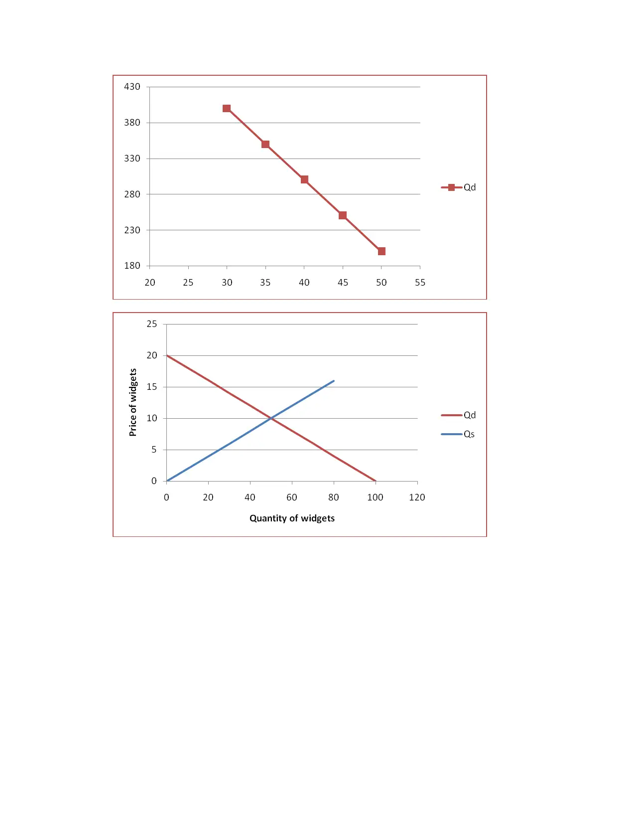
Qd= 100-5P
Qs = 5P
c. Equilibrium is shown where demand (Qd) equals supply.(Qs)
100 – 5P = 5P
10P = 100
P= 10 and Q= 5*10=50
d. Consumer surplus = ½ *50*(20-10) = 250
Producer surplus = ½ *50*10 = 250
Total surplus = 500
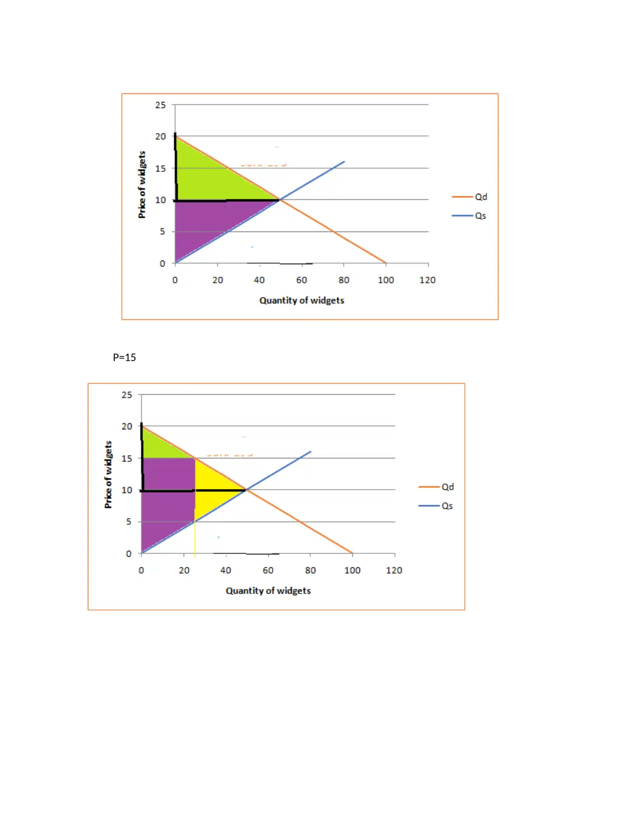
e. At a price of $15 we do not have free equilibrium as demand < supply. So the quantity in this
constrained equilibrium will be Qd. To get Qd we put P = 15 in Qd and get Q= 100-5*15 =25
Using this we calculate surplus with Q= 25 and P = 15.
The consumer surplus is = ½*25*(20-15) = 62.5.
Producer surplus = (15-5)*25 + ½ *5*25 = 212.5 total = 275.
Deadweight loss = ½ *(15-5)*25 = 125
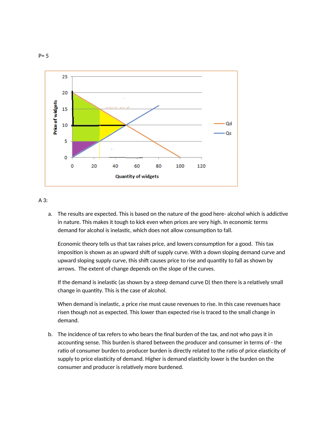
The same logic can be followed for a price of $5. As supply < demand we end up with a
constrained equilibrium, where quantity is given by Qs or 5*5 = 25. Using P= 5 and Q= 25 we get
Consumer surplus = = (15-5)*25 + ½ *5*25 = 212.5.
Producer surplus = ½ *5*25 = 62.5.
Deadweight loss = ½ *(15-5)*25 = 125.
f. Diagrams are shown below with green area for consumer surplus and purple for producer
surplus and yellow for deadweight loss

P=15

P= 5
A 3:
a. The results are expected. This is based on the nature of the good here- alcohol which is addictive
in nature. This makes it tough to kick even when prices are very high. In economic terms
demand for alcohol is inelastic, which does not allow consumption to fall.
Economic theory tells us that tax raises price, and lowers consumption for a good. This tax
imposition is shown as an upward shift of supply curve. With a down sloping demand curve and
upward sloping supply curve, this shift causes price to rise and quantity to fall as shown by
arrows. The extent of change depends on the slope of the curves.
If the demand is inelastic (as shown by a steep demand curve D) then there is a relatively small
change in quantity. This is the case of alcohol.
When demand is inelastic, a price rise must cause revenues to rise. In this case revenues hace
risen though not as expected. This lower than expected rise is traced to the small change in
demand.
b. The incidence of tax refers to who bears the final burden of the tax, and not who pays it in
accounting sense. This burden is shared between the producer and consumer in terms of - the
ratio of consumer burden to producer burden is directly related to the ratio of price elasticity of
supply to price elasticity of demand. Higher is demand elasticity lower is the burden on the
consumer and producer is relatively more burdened.

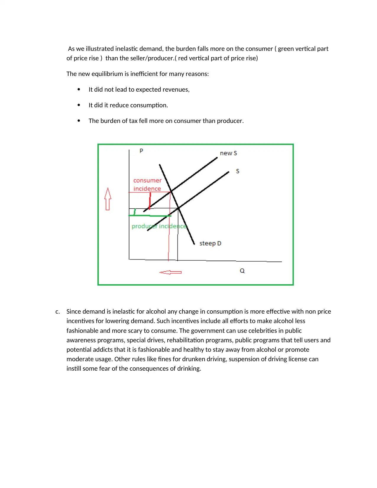
As we illustrated inelastic demand, the burden falls more on the consumer ( green vertical part
of price rise ) than the seller/producer.( red vertical part of price rise)
The new equilibrium is inefficient for many reasons:
 It did not lead to expected revenues,
 It did it reduce consumption.
 The burden of tax fell more on consumer than producer.
c. Since demand is inelastic for alcohol any change in consumption is more effective with non price
incentives for lowering demand. Such incentives include all efforts to make alcohol less
fashionable and more scary to consume. The government can use celebrities in public
awareness programs, special drives, rehabilitation programs, public programs that tell users and
potential addicts that it is fashionable and healthy to stay away from alcohol or promote
moderate usage. Other rules like fines for drunken driving, suspension of driving license can
instill some fear of the consequences of drinking.

REFERENCES
Anon., n.d. Shifts in demand and supply. [Online] Available at:
https://cnx.org/contents/ETAPPz5d@5/Shifts-in-Demand-and-Supply-fo [Accessed 3 Sep 2017].
CSun.edu, n.d. Microeconomics. [Online] Available at:
http://www.csun.edu/sites/default/files/micro3.pdf [Accessed 8 Sep 2017].
Econ.ohio-state.edu, n.d. Elasticity. [Online] Available at
http://www.econ.ohio-state.edu/jpeck/H200/EconH200L5.pdf [Accessed 3 Sep 2017].