BUS105 Computing Assignment: Excel Data Analysis and Interpretation

This BUS105 computing assignment utilizes Microsoft Excel to perform data analysis, covering various techniques such as defining key terms, conducting regression analysis, creating charts, and generating pivot tables. The assignment involves using data to develop equations, calculate Z-scores using wolframalpha.com, and determine p-values through comparison of means. It includes sections on data summarization, finding patterns in datasets, and interpreting results from different statistical analyses. The student explores concepts like categorical variables, histograms, scatterplots, and back-to-back histograms to visualize and interpret data relationships. The assignment culminates in the explanation of p-values and the rejection of null hypotheses based on the analysis, with references to relevant literature on Excel data analysis.

Running Head: BUS105 COMPUTING ASSIGNMENT
Bus105 computing assignment
Name: Paras Bhandari
Student number: 1600712
Sample ID: 238

The assignment is based on the use of Excel to generate charts. Section one involves defining
useful terms to be used in Ms Excel. Section two uses data to do regression. Using the line of best fit,
an equation is developed and used to find different estimates. In this section, there is the use of
wolframalpha.com to get the different values of Zscore. The consequent sections utilizes Ms Excel to
come up with pivot tables and use comparisons of means to come up with the p-values.
Section one
A dataset can be expounded as a collection of info that is related in one way or the next. One unique
thing about a dataset is the fact that a dataset can be manipulated as a single unit by a computer while
carrying out computations.
Categorical variable: This is a variable that can go up against one of a restricted, and generally settled,
number of conceivable values, assigning every individual or other unit of observation to a specific
group or nominal classification based on some subjective property.
A nominal variable can be explained as a categorical variable that lacks any significant order. In
contrast, an ordinal variable can be said to be a categorical variable that possess a significant order.
A ratio variable can be defined as a quantitative variable where a value of 0 does not amount to
anything significant, for example, measure of power utilized.
An interval variable on the other hand also qualifies as a quantitative variable only that in this case a
value of 0 amounts to something significant, for example 00 Celsius.
*Summarizing variables and the relationship(s) between them
Histograms, Zscores, bar graphs, pivot tables and other charts are examples of useful outputs
that can help describe relationships among different sets of data.
*Why is important to be able to find patterns in a dataset using a computer
Patterns are important in studying the relation between the data and be able to use these data to
make life and business decisions that are well informed. Tables alone with different datasets are not

enough for us to visualize these patterns. For instance, In a scatterplot, two measurements are mapped
to the x-and y-axes. You can even show a third measurement to the shading or size of the showed
images. Line outlines are particularly suited for demonstrating fleeting developments while bar graphs
are ideal for looking at all out information. You can stack diagram components over each other. On the
off chance that you need to look at few groups in your information, showing numerous occurrences of
a similar diagram is a capable way. In all outlines you can utilize various types of scales to investigate
distinctive viewpoints in your information.
Section two
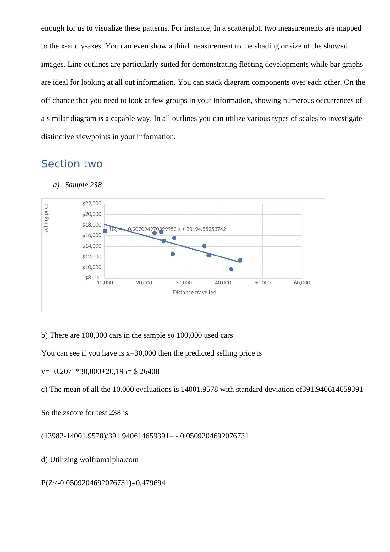
a) Sample 238
10,000 20,000 30,000 40,000 50,000 60,000
$8,000
$10,000
$12,000
$14,000
$16,000
$18,000
$20,000
$22,000
f(x) = − 0.207094970399953 x + 20194.55253742
Distance travelled
selling price
b) There are 100,000 cars in the sample so 100,000 used cars
You can see if you have is x=30,000 then the predicted selling price is
y= -0.2071*30,000+20,195= $ 26408
c) The mean of all the 10,000 evaluations is 14001.9578 with standard deviation of391.940614659391
So the zscore for test 238 is
(13982-14001.9578)/391.940614659391= - 0.0509204692076731
d) Utilizing wolframalpha.com
P(Z<-0.0509204692076731)=0.479694

e) So in the event that you contrast test 238 with the 10,000 samples at that point
Anticipated rank = P(Z<zscore)*10000=0.479694*10,000= $4796.94

Section three
a)
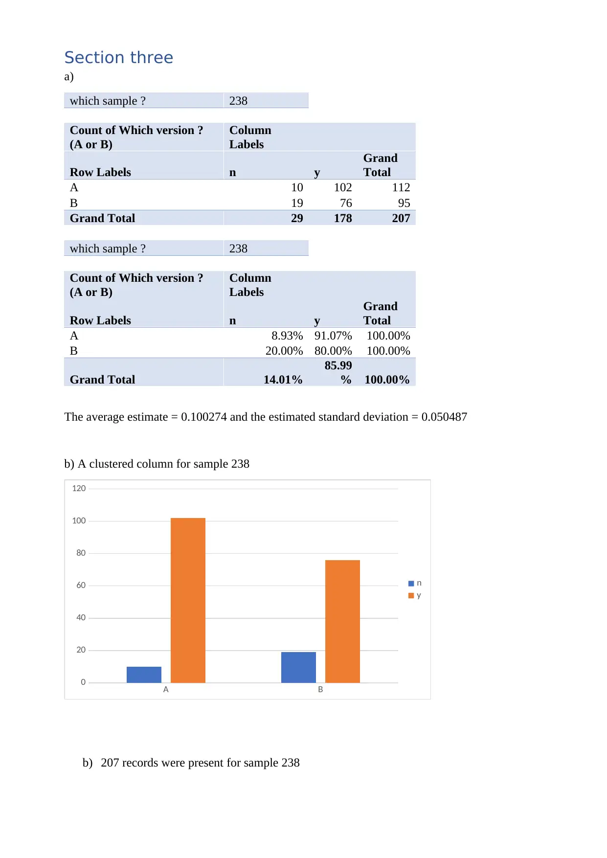
which sample ? 238
Count of Which version ?
(A or B)
Column
Labels
Row Labels n y
Grand
Total
A 10 102 112
B 19 76 95
Grand Total 29 178 207
which sample ? 238
Count of Which version ?
(A or B)
Column
Labels
Row Labels n y
Grand
Total
A 8.93% 91.07% 100.00%
B 20.00% 80.00% 100.00%
Grand Total 14.01%
85.99
% 100.00%
The average estimate = 0.100274 and the estimated standard deviation = 0.050487
b) A clustered column for sample 238
A B
0
20
40
60
80
100
120
n
y
b) 207 records were present for sample 238

c)
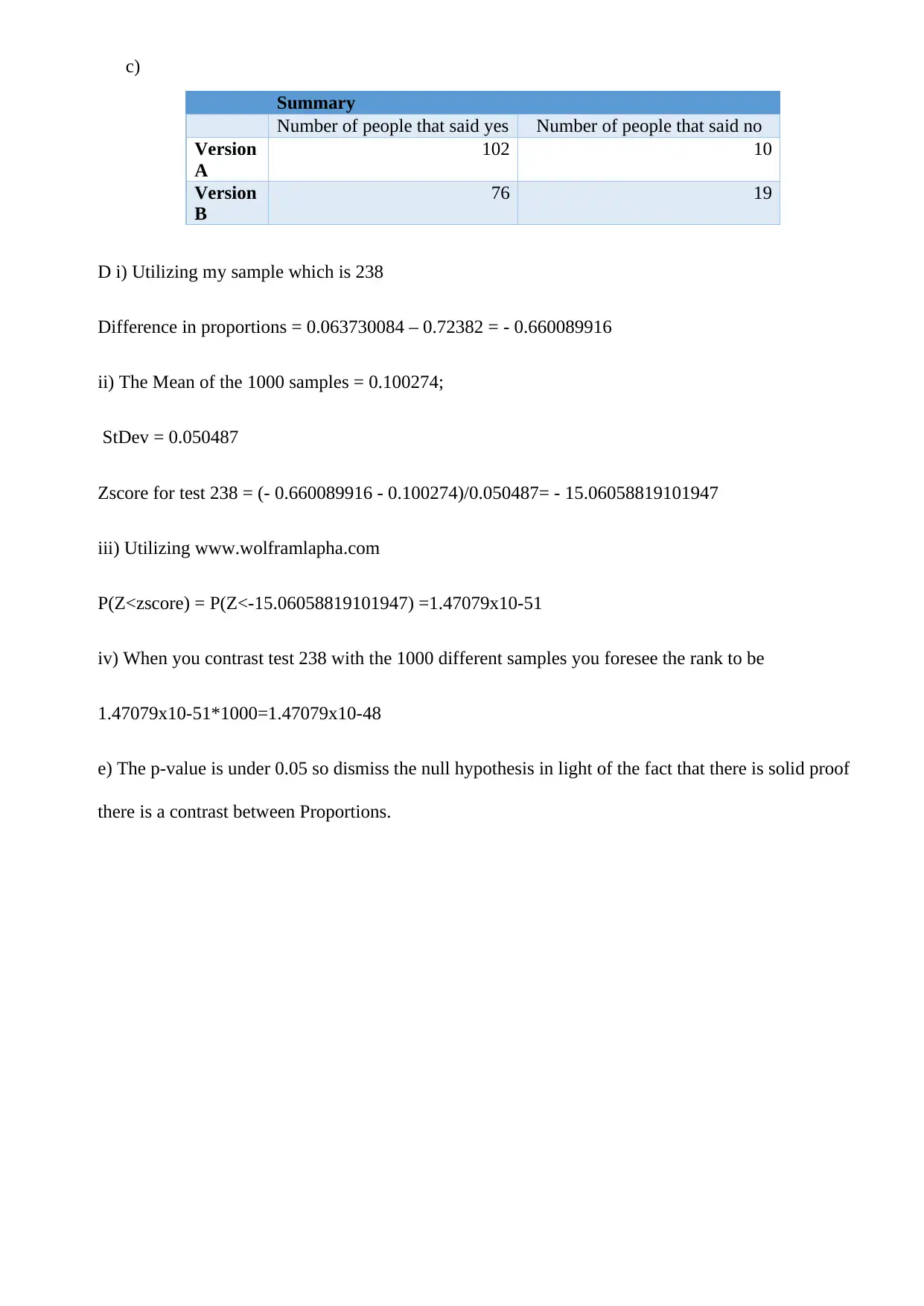
Summary
Number of people that said yes Number of people that said no
Version
A
102 10
Version
B
76 19
D i) Utilizing my sample which is 238
Difference in proportions = 0.063730084 – 0.72382 = - 0.660089916
ii) The Mean of the 1000 samples = 0.100274;
StDev = 0.050487
Zscore for test 238 = (- 0.660089916 - 0.100274)/0.050487= - 15.06058819101947
iii) Utilizing www.wolframlapha.com
P(Z<zscore) = P(Z<-15.06058819101947) =1.47079x10-51
iv) When you contrast test 238 with the 1000 different samples you foresee the rank to be
1.47079x10-51*1000=1.47079x10-48
e) The p-value is under 0.05 so dismiss the null hypothesis in light of the fact that there is solid proof
there is a contrast between Proportions.

Section four
a)
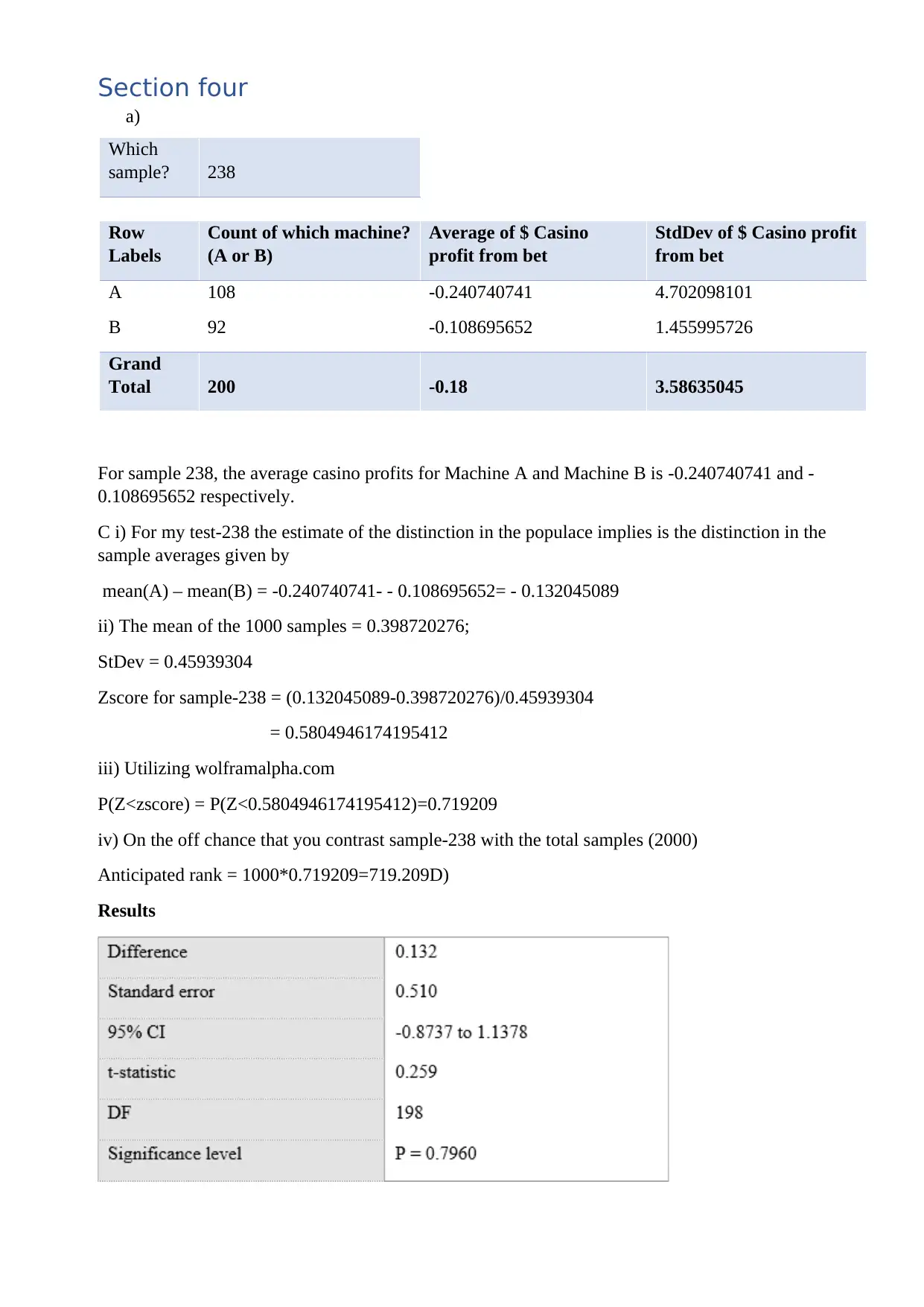
For sample 238, the average casino profits for Machine A and Machine B is -0.240740741 and -
0.108695652 respectively.
C i) For my test-238 the estimate of the distinction in the populace implies is the distinction in the
sample averages given by
mean(A) – mean(B) = -0.240740741- - 0.108695652= - 0.132045089
ii) The mean of the 1000 samples = 0.398720276;
StDev = 0.45939304
Zscore for sample-238 = (0.132045089-0.398720276)/0.45939304
= 0.5804946174195412
iii) Utilizing wolframalpha.com
P(Z<zscore) = P(Z<0.5804946174195412)=0.719209
iv) On the off chance that you contrast sample-238 with the total samples (2000)
Anticipated rank = 1000*0.719209=719.209D)
Results
Which
sample? 238
Row
Labels
Count of which machine?
(A or B)
Average of $ Casino
profit from bet
StdDev of $ Casino profit
from bet
A 108 -0.240740741 4.702098101
B 92 -0.108695652 1.455995726
Grand
Total 200 -0.18 3.58635045

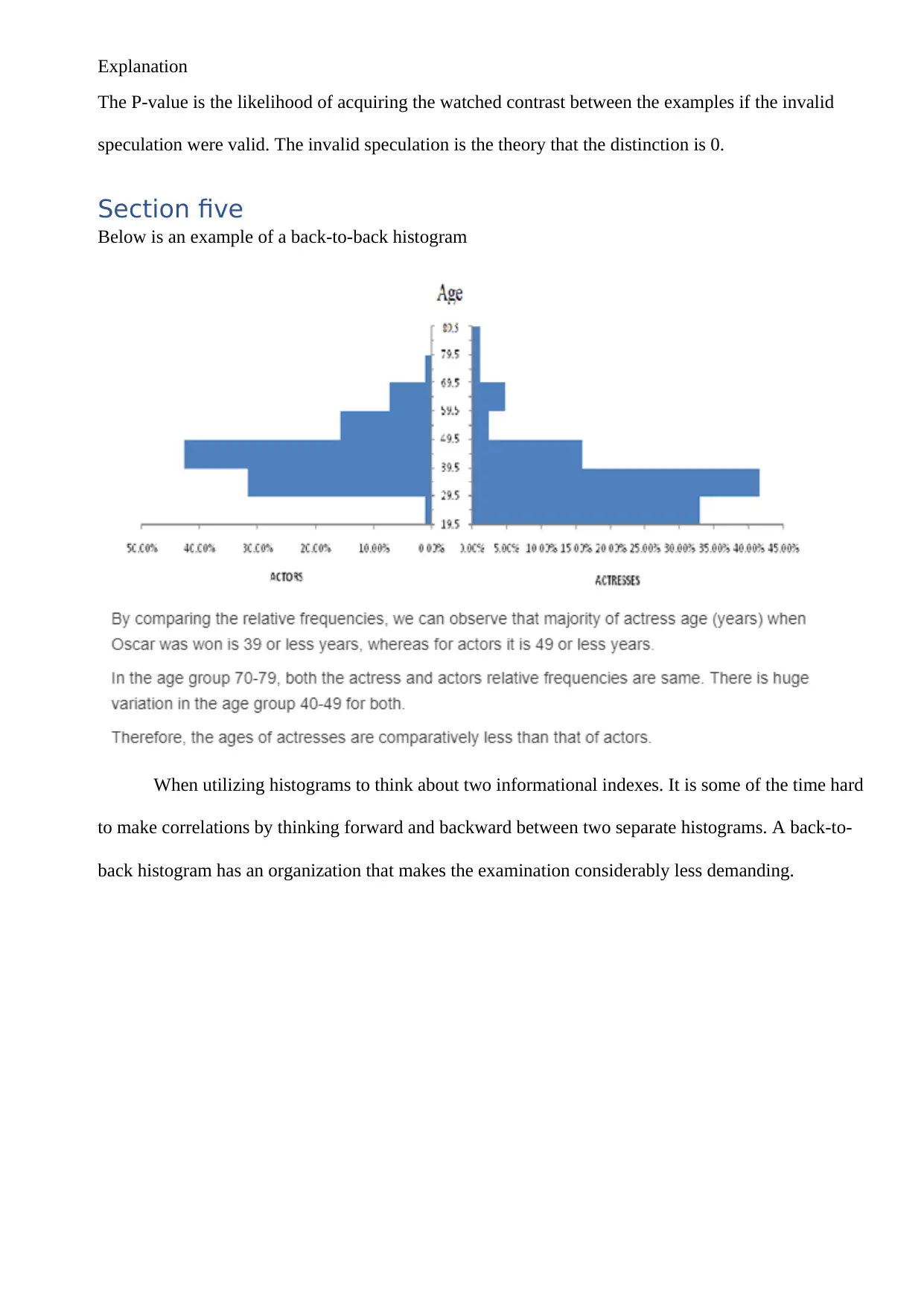
Explanation
The P-value is the likelihood of acquiring the watched contrast between the examples if the invalid
speculation were valid. The invalid speculation is the theory that the distinction is 0.
Section five
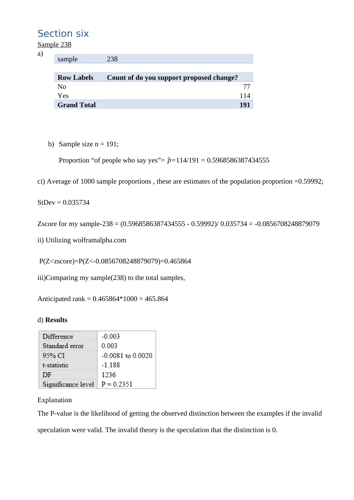
Below is an example of a back-to-back histogram
When utilizing histograms to think about two informational indexes. It is some of the time hard
to make correlations by thinking forward and backward between two separate histograms. A back-to-
back histogram has an organization that makes the examination considerably less demanding.

Section six
Sample 238
a)
b) Sample size n = 191;
Proportion “of people who say yes”= ^p=114/191 = 0.5968586387434555
ci) Average of 1000 sample proportions , these are estimates of the population proportion =0.59992;
StDev = 0.035734
Zscore for my sample-238 = (0.5968586387434555 - 0.59992)/ 0.035734 = -0.0856708248879079
ii) Utilizing wolframalpha.com
P(Z<zscore)=P(Z<-0.0856708248879079)=0.465864
iii)Comparing my sample(238) to the total samples,
Anticipated rank = 0.465864*1000 = 465.864
d) Results
Explanation
The P-value is the likelihood of getting the observed distinction between the examples if the invalid
speculation were valid. The invalid theory is the speculation that the distinction is 0.
sample 238
Row Labels Count of do you support proposed change?
No 77
Yes 114
Grand Total 191

References
Miller, A. (2014). Introduction to Using Excel Pivot Tables and Pivot Charts to Increase Efficiency in
Library Data Analysis and Illustration. Journal Of Library Administration, 54(2), 94-106.
doi:10.1080/01930826.2014.903365
Jelen, B. (2010). Filtering Multiple Pivot Tables in Excel 2010. Strategic Finance, 92(3), 52.
Chiaramonte, L., Croci, E., & Poli, F. (2015). Should we trust the Z-score? Evidence from the
European
Banking Industry. Global Finance Journal, 28111-131. doi:10.1016/j.gfj.2015.02.002