BUS105 Computing Assignment Report

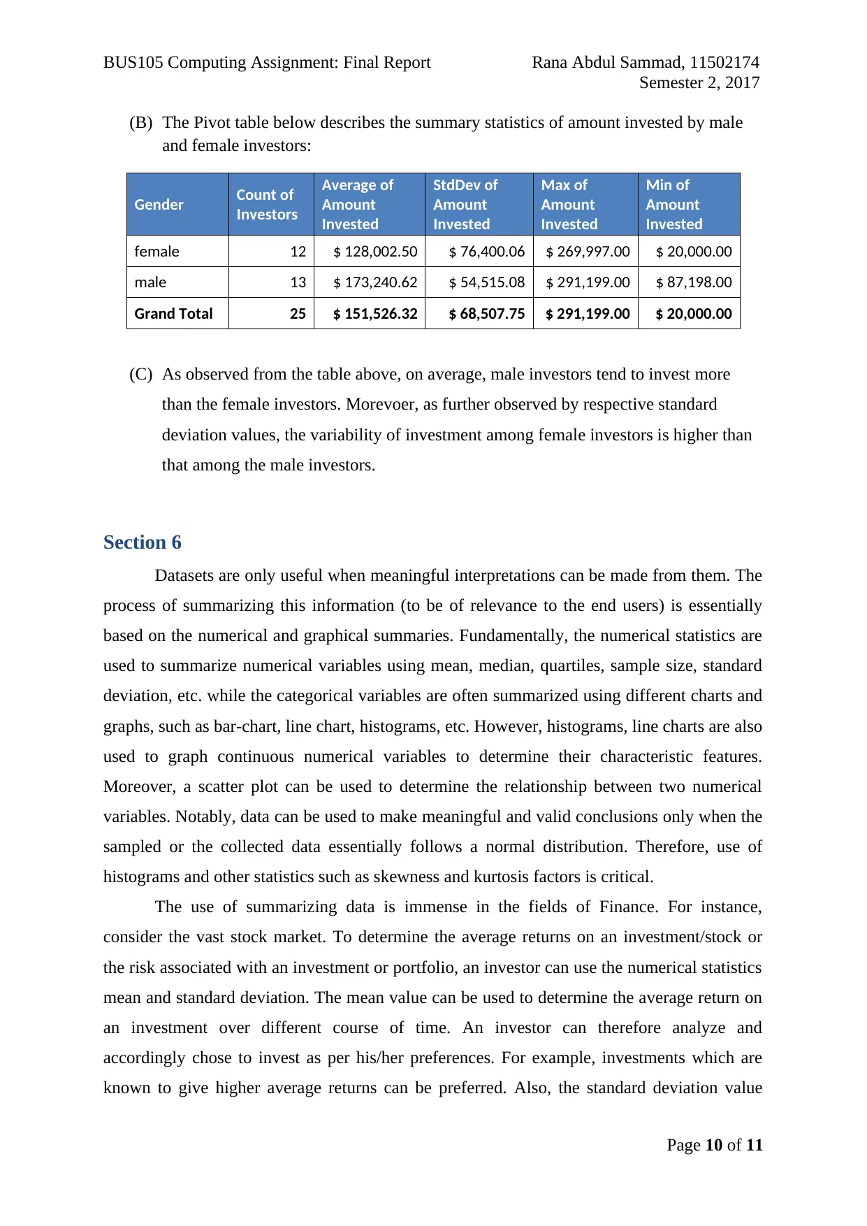
This report presents a comprehensive analysis of various datasets using statistical methods. It begins with a scatter plot analysis to determine the relationship between annual income and savings contributions, followed by the creation of pivot tables to analyze investment risk and profitability. Hypothesis testing is employed to compare the proportions of losses between high-risk and low-risk investments, and a z-test is used to compare the mean returns of these investments. A confidence interval is calculated for the proportion of people supporting a business change based on an opinion poll. Finally, the report includes a descriptive analysis of a dataset on investor gender and investment amounts, summarizing the data using descriptive statistics and pivot tables. The report concludes by discussing the importance of data summarization and its applications in finance, using examples of mean and standard deviation in investment analysis. The report includes references to external resources used for guidance and further explanation.

Running Head: BUS105 COMPUTING ASSIGNMENT: FINAL REPORT
Student Name:
Student ID:
Course:
Professor Name:
Date Submitted:
BUS105 Computing Assignment: Final Report
Semester 2, 2017
Allocated Sample Number: 7
Page 1 of 11

BUS105 Computing Assignment: Final Report Rana Abdul Sammad, 11502174
Semester 2, 2017
Section 1
(A) Scatter Plot:
$50,000 $100,000 $150,000 $200,000 $250,000 $300,000
$5,000
$15,000
$25,000
$35,000
$45,000
$55,000
$65,000
f(x) = 0.166804724984862 x − 4018.18192231845
Scatter Plot between Income and Annual Contribution
to Savings
Income
annual contribution
As observed from the scatter plot above, a linear, positive slope relationship exists
between the two numerical variables. Therefore, it can be stated that the annual
contribution to savings (in $) increases with an increase in annual income (in $) and
decreases with a decrease in annual income.
(B) The regression equation for the above model is given by:
y=0.1668 x−4018.2
where x=Income($) and y= Annual contribution¿ savings($)
Therefore, for an annual income of $200,000:
Annual Contribution y=0.1668 ( 200000 )−4018.2
y=$ 29,341.8
(C) Given that μ=$ 27,000 and σ =$ 2,100
Therefore, z-score is computed as:
z= x−μ
σ = 29341.8−27000
2100 ≈1.12
(D) Using an online calculator P ( Z <1.12 ) =0.8676
Page 2 of 11

BUS105 Computing Assignment: Final Report Rana Abdul Sammad, 11502174
Semester 2, 2017
(E) Expected rank = P(Z< 1.12) ×10000
≈ 0.8676 ×10000
≈ 86760
Section 2
(A) The overall combined Pivot table below describes the proportion of high risk (riskier
type) investments that made a loss ^p1 and also the proportion of low risk (safer type)
investments that made a loss ^p2:
Investment Type/Proportion of Profit and Loss Column Labels
Row Labels Loss Profit Grand Total
risky 0.20 0.80 1.00
safe 0.17 0.83 1.00
Grand Total 0.19 0.81 1.00
As observed, ^p1=0.20 while ^p2=0.17
(B) Comparison Bar Chart:
(C) As observed from the Pivot table and the bar-chart above, overall, high risk (or risky)
investments have a comparatively lesser chance to make a profit than low-risk or
safer investments.
(D) ^p1− ^p2 is the point estimate of p1− p2, computed as:
⟹ ^p1− ^p2=0.20−0.17=0.03
Page 3 of 11

BUS105 Computing Assignment: Final Report Rana Abdul Sammad, 11502174
Semester 2, 2017
Accordingly, z-score is:
z= 0.03−0.1
0.0743 ≈−0.942
Therefore, using online calculator P ( Z <−0.942 ) =0.1731
Expected rank = P(Z<−0.942) × 4000
≈ 0. 1731× 4000
≈ 692
(E) The hypotheses are stated as:
Null H0 : p1− p2=0 i . e . p1=p2
Alternative Ha : p1− p2 ≠ 0 i . e . p1 ≠ p2
Here, p1− p2 is the hypothesized difference of population proportions. The null
hypothesis is rejected if the difference is statistically significant at a significance level
of 5%, i.e. for α=0.05.
To test the hypothesis, a two-tailed (non-directional) z-test is used.
Further, following information is computed in Excel:
Investment Type/COUNT of Profit and Loss Column Labels
Row Labels Loss Profit Grand Total
risky 14 56 70
safe 5 25 30
Grand Total 19 81 100
Uisng the above table and information from part A above, the respective values are
put in the online calculator (http://epitools.ausvet.com.au/content.php?page=z-test-2).
Obtained results are summarized below:
Page 4 of 11

BUS105 Computing Assignment: Final Report Rana Abdul Sammad, 11502174
Semester 2, 2017
Since the p-value¿ 0.7265>0.05=α, the null hypothesis cannot be rejected.
Therefore, it can be stated that there is insufficient evidence to claim that that the two
population proportions are equal. In other words, it can be said that the proportion of
high risk investments that made a loss ^p1 and the proportion of low risk investments
that made a loss ^p2 are not equal, i.e. are statistically different to each other.
Section 3
(A) The Pivot table below describes the summary statisitics of Returns on high risk and
low risk investments:
High Risk? Count Average return StdDev of returns
no 64 0.0347 0.0032
yes 36 0.0589 0.0988
Grand Total 100 0.0434 0.0600
As observed, x1=0.0347 while x2=0. 0589
n1=64 while n2 =36
s1=0.0032 while s2=0.0988
Page 5 of 11

BUS105 Computing Assignment: Final Report Rana Abdul Sammad, 11502174
Semester 2, 2017
(B) Following additional five-number summary was computed for the given returns data:
Returns Low Risk High Risk
Minimum 0.030 -0.100
Quartile 1 0.032 -0.020
Median 0.035 0.050
Quartile 3 0.037 0.130
Maximum 0.040 0.220
Comparison Bar Chart:
(C) As observed from the above summary statistics table and the chart above, on
avaerage, the returns on high-risk investments are higher than the returns on low risk
investments. However, the variability of returns is comparitively higher for the high-
risk investments.
(D) By definition, the difference x1−x2 is the point estimate of μ1−μ2, computed as:
⟹ x1 −x2=0.0347−0.0589=−0.0242
Further, it is given that μd =−0.0256 and σ d=0.0173
Accordingly, z-score is:
z=−0.0242−(−0.0256)
0.0173 ≈ 0.081
Therefore, using online calculator P ( Z <0.081 ) =0.5323
Page 6 of 11

BUS105 Computing Assignment: Final Report Rana Abdul Sammad, 11502174
Semester 2, 2017
Expected rank = P( Z<0.081)×2 000
≈ 0. 5323× 2 000
≈ 1065
(E) The hypotheses are stated as:
Null H0 : μ1−μ2=0i . e . μ1=μ2
Alternative Ha : μ1−μ2 ≠ 0i . e . μ1 ≠ μ2
Here, μ1−μ2 is the hypothesized difference of population means. The null hypothesis
is rejected if the mean of two populations (i.e. mean of returns on high-risk and low-
risk investments) are statistically different at the given significance level of 5%, i.e.
for α=0.05.
To test the hypothesis, a two-tailed (non-directional) z-test is used.
As computed above, the following table describes the summary statistics paramters
required to test the hypothesis:
High Risk? Count Average return StdDev of returns
no 64 0.0347 0.0032
yes 36 0.0589 0.0988
Grand Total 100 0.0434 0.0600
Uisng the online calculator
(https://www.medcalc.org/calc/comparison_of_means.php), following results are
obtained:
Since the p-value¿ 0. 0522>0.05=α, the null hypothesis cannot be rejected.
Therefore, it can be stated that there is insufficient evidence to claim that that the two
population means are equal. In other words, it can be said that the mean returns of
high-risk and low-risk investments are not equal to each other.
Page 7 of 11

BUS105 Computing Assignment: Final Report Rana Abdul Sammad, 11502174
Semester 2, 2017
Section 4
(A) The following Pivot table describes the number of people that answered ‘no’ and the
number of people that answered ‘yes’ in an opinion poll conducted by a business to
find out if the customers support a change to the Business:
Opinion Count of do you support
proposed change?
Proportion of do you support
proposed change?
no 81 0.3699
yes 138 0.6301
Grand Total 219 1.00
(B) The sample size (i.e. number) of people who support the change is 138. This is
equivalent to about 63.01% of the sampled population. In notations,
n yes=138
^pyes=0.6301
Here, ^pyes is the point estimate for the population proportion pyes, i.e. the proportion
of people who support the change.
(C) Using the given information in the question and the above computations:
z= 0.6 301−0.6
0.0357 ≈ 0.843
Therefore, using online calculator P ( Z <0. 843 ) =0.8004
Expected rank = P( Z<0. 843) ×1 000
≈ 0.8004 × 1000
≈ 800
(D) As computed above, about 63.01% of the sampled population support the change. i.e.
^pyes=0.6301
Therefore, the confidence interval of a population proportion p who support the
change is given by:
^pyes ± zα/ 2 ( √ ^pyes ( 1− ^pyes )
ntotal )
For 95% confidence level zα / 2=1. 96. Substituting the values gives:
Page 8 of 11

BUS105 Computing Assignment: Final Report Rana Abdul Sammad, 11502174
Semester 2, 2017
¿ 0.6301 ±1.96 ( √ 0.6301 ( 1−0.6301 )
219 )
¿ 0.6301 ±1.96 (0.0326)
¿ 0.6301 ±0. 0639
¿ ( 0.5662 , 0.694 ) ∨(56.62 % , 69.4 %)
Therefore, the 95% confidence interval for the proportion of people that support the
change is ( 0.5662 , 0.694 ).
Section 5
(A) Descroption of the sampled dataset:
The following sampled data for 25 investors describes the gender of the investor and
the amount invested by them. The two variables being measured are:
 Categorical Variable: Gender (Male/Female)
 Numerical Variable: Amount Invested (in $)
Dataset:
Gender Amount
Invested Gender Amount
Invested Gender Amount
Invested
female $ 52,899 male $ 87,198 female $ 269,997
male $ 136,798 female $ 196,097 female $ 86,749
male $ 164,598 female $ 44,499 male $ 291,199
male $ 137,348 male $ 251,898 female $ 62,998
female $ 197,998 male $ 149,599 female $ 145,999
male $ 227,998 male $ 134,498 female $ 160,198
male $ 174,999 male $ 161,949 female $ 20,000
male $ 156,998 female $ 117,398 female $ 181,198
male $ 177,048
Page 9 of 11

BUS105 Computing Assignment: Final Report Rana Abdul Sammad, 11502174
Semester 2, 2017
(B) The Pivot table below describes the summary statistics of amount invested by male
and female investors:
Gender Count of
Investors
Average of
Amount
Invested
StdDev of
Amount
Invested
Max of
Amount
Invested
Min of
Amount
Invested
female 12 $ 128,002.50 $ 76,400.06 $ 269,997.00 $ 20,000.00
male 13 $ 173,240.62 $ 54,515.08 $ 291,199.00 $ 87,198.00
Grand Total 25 $ 151,526.32 $ 68,507.75 $ 291,199.00 $ 20,000.00
(C) As observed from the table above, on average, male investors tend to invest more
than the female investors. Morevoer, as further observed by respective standard
deviation values, the variability of investment among female investors is higher than
that among the male investors.
Section 6
Datasets are only useful when meaningful interpretations can be made from them. The
process of summarizing this information (to be of relevance to the end users) is essentially
based on the numerical and graphical summaries. Fundamentally, the numerical statistics are
used to summarize numerical variables using mean, median, quartiles, sample size, standard
deviation, etc. while the categorical variables are often summarized using different charts and
graphs, such as bar-chart, line chart, histograms, etc. However, histograms, line charts are also
used to graph continuous numerical variables to determine their characteristic features.
Moreover, a scatter plot can be used to determine the relationship between two numerical
variables. Notably, data can be used to make meaningful and valid conclusions only when the
sampled or the collected data essentially follows a normal distribution. Therefore, use of
histograms and other statistics such as skewness and kurtosis factors is critical.
The use of summarizing data is immense in the fields of Finance. For instance,
consider the vast stock market. To determine the average returns on an investment/stock or
the risk associated with an investment or portfolio, an investor can use the numerical statistics
mean and standard deviation. The mean value can be used to determine the average return on
an investment over different course of time. An investor can therefore analyze and
accordingly chose to invest as per his/her preferences. For example, investments which are
known to give higher average returns can be preferred. Also, the standard deviation value
Page 10 of 11

BUS105 Computing Assignment: Final Report Rana Abdul Sammad, 11502174
Semester 2, 2017
(say, for weekly, monthly, or yearly data of returns) can describe the variability of returns to
the mean value. This variability can describe for an investment is either risky or safer to invest
in. For example, a risky investment will have a higher variability among its return values, i.e.
a higher standard deviation. Accordingly, an investor can choose to be risk averse or a risk
taker as per his/her investment preference.
References
1. Guide to summarizing datasets
https://app.box.com/s/jxuqhpzjrfj14xiq28x1bnywjv1iayr4
2. Discussion of how mean and standard deviation is used in finance
https://www.youtube.com/watch?v=UwO4JvB9OpE
Page 11 of 11