BUS5DWR Assignment: Census Data Wrangling and Analysis with R

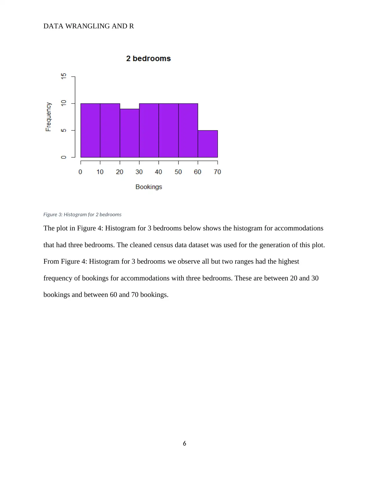
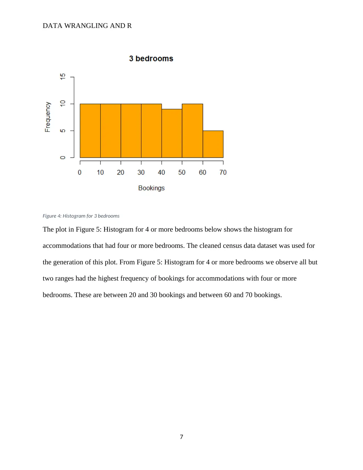
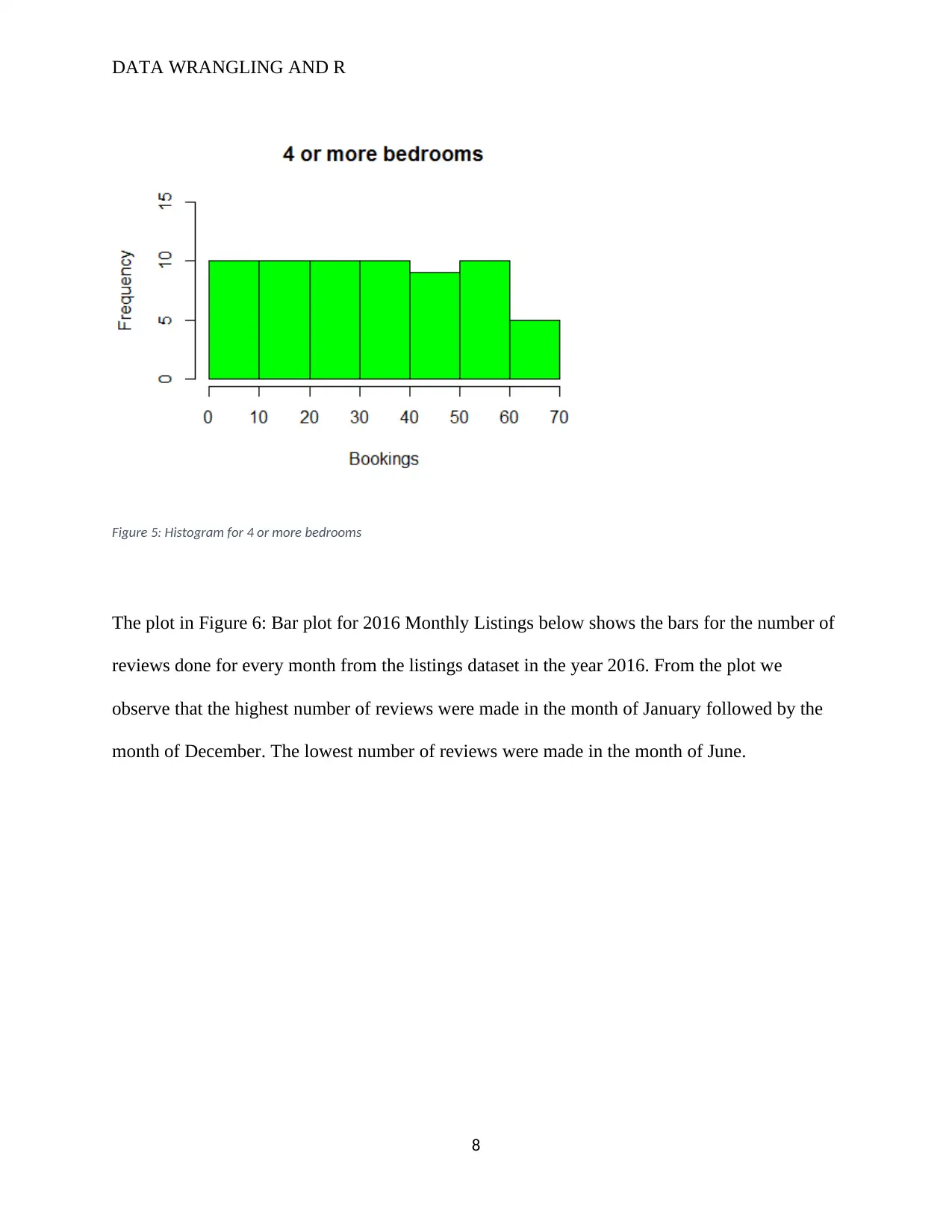
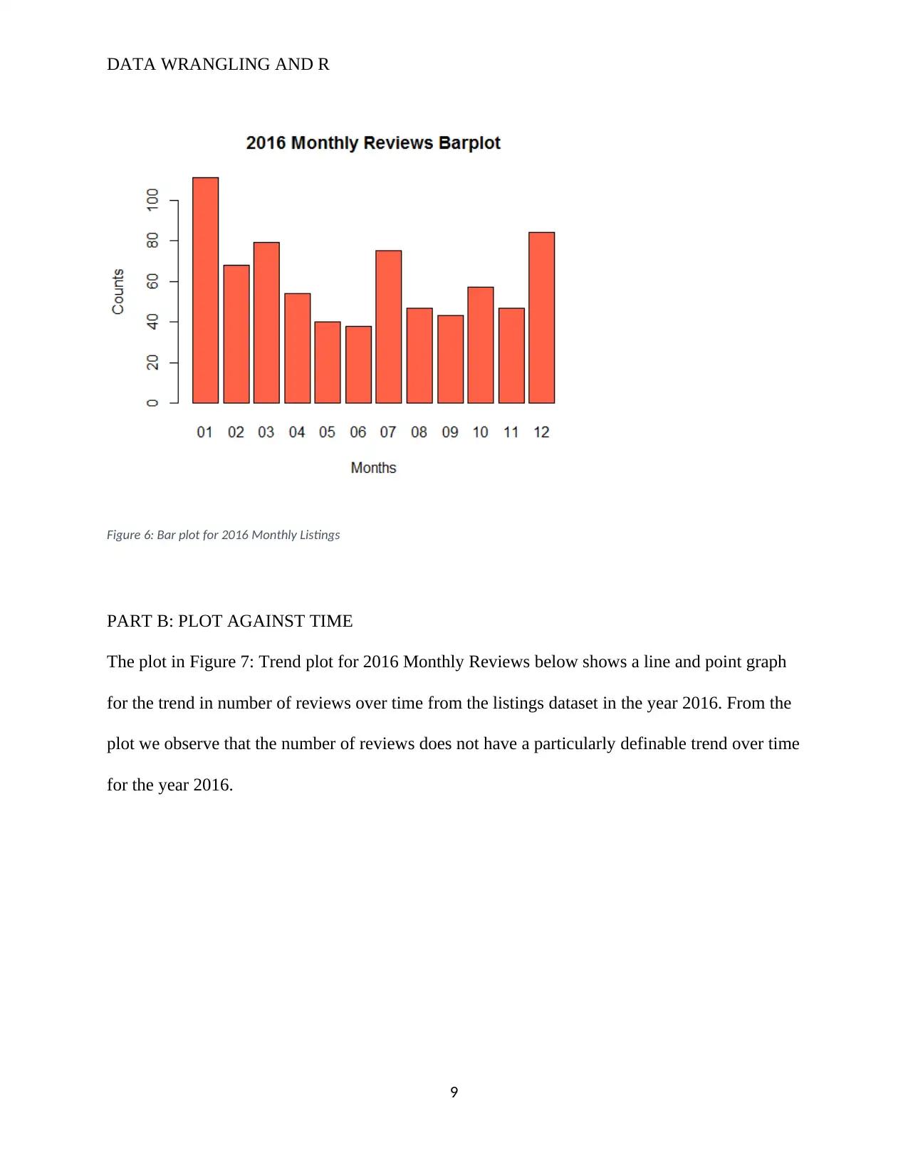
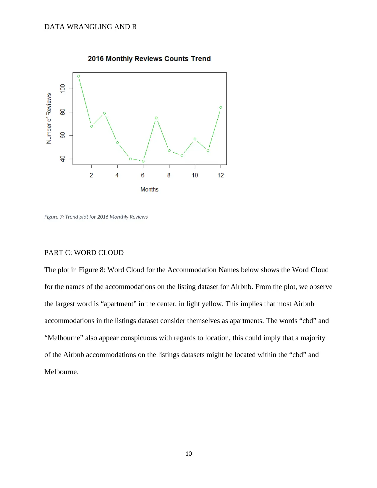
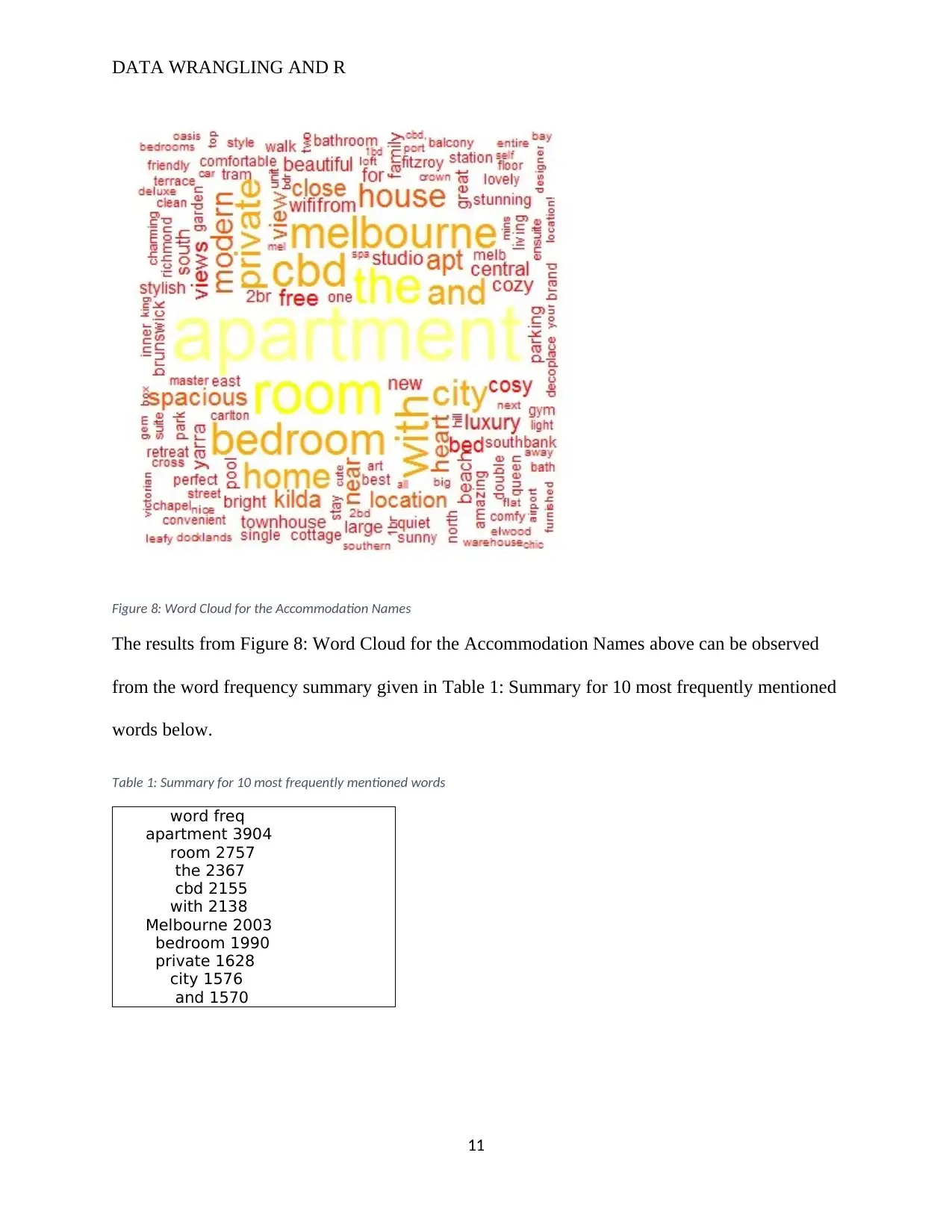
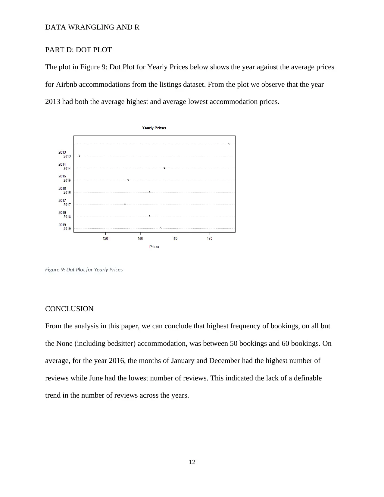
This assignment focuses on data wrangling and visualization using R, specifically applied to census data and listings datasets to analyze accommodation trends in Melbourne. The initial part of the assignment addresses the concept of 'tidy' data and explains why the census data is considered 'untidy' due to its structure. The subsequent sections involve creating various data visualizations, including histograms for different bedroom counts, bar plots for monthly listings, trend plots for monthly reviews, word clouds for accommodation names, and dot plots for yearly prices. The analysis reveals insights such as the frequency of bookings for different accommodation types, trends in monthly reviews, and the prevalence of apartments in Airbnb listings. The assignment concludes by summarizing the key findings and observations derived from the visualizations, emphasizing the usefulness of R in data analysis.

DATA WRANGLING AND R

DATA WRANGLING AND R
Table of Contents
INTRODUCTION.......................................................................................................................................3
DATA ANALYSIS.....................................................................................................................................3
DATA “TIDINESS” OF CENSUS DATA..............................................................................................3
PART A: HISTOGRAMS AND BARPLOTS.........................................................................................4
PART B: PLOT AGAINST TIME..........................................................................................................9
PART C: WORD CLOUD....................................................................................................................10
PART D: DOT PLOT............................................................................................................................12
CONCLUSION.........................................................................................................................................12
References.................................................................................................................................................14
2

DATA WRANGLING AND R
INTRODUCTION
Data visualization refers to a data analysis technique that provides for the graphing of the results
of an analysis for easier interpretation (Kirk, 2016). Data visualization tools simplify the
communication of the findings of a research especially if the audience is not well familiarized
with statistics related terminologies and tests (Roles, Baeten & Signer 2016). In general, through
data visualization research finding are made more understandable to the end users.
This paper focuses in applying data visualization tools for the census data and listings datasets.
The aim of the analysis in the study is to graphical analyze the various variables in the census
data and listing datasets. The census data dataset contains information about the accommodations
in private dwellings in various areas of Melbourne for the years 2011 and 2016. The listings
dataset on the other hand contains information about the Airbnb accommodations in Melbourne
from the year 2011 through to the year 2019.
The analysis is this research paper provides visualization of the accommodation trends for the
city of Melbourne according to the two datasets; census data and listings datasets.
DATA ANALYSIS
DATA “TIDINESS” OF CENSUS DATA
The census data is considered as “untidy” due to the data recording method used. The data for
each area was recorded separately and as columns with the parameters set as rows. This is in
contrast to cleaned, prepared and “tidy” data that have observations recorded continuously and
row-wise, and the parameters arranged column-wise. Hence the census data is not “tidy”
3

DATA WRANGLING AND R
PART A: HISTOGRAMS AND BARPLOTS
The plot in Figure 1: Histogram of None (Includes bedsitters) below shows the histogram for
accommodations that had no bedrooms, that is number of bedrooms equaled 0. These
accommodations also included the bedsitters. The cleaned census data dataset was used for the
generation of this plot. From Figure 1: Histogram of None (Includes bedsitters) we observe that
the highest frequency of bookings for accommodations with no bedrooms was between 0 and 10.
The ranges with the joint lowest frequency of bookings were between 20 and 30 bookings,
between 30 and 40 bookings, and between 50 and 60 bookings.
Figure 1: Histogram of None (Includes bedsitters)
The plot in Figure 2: Histogram for 1 bedroom below shows the histogram for accommodations
that had one room. The cleaned census data dataset was used for the generation of this plot. From
Figure 2: Histogram for 1 bedroom we observe that the highest frequency of bookings for
4

DATA WRANGLING AND R
accommodations one bedroom was between 50 and 60. We also observe that the lowest
frequency of bookings was between 60 and 70.
Figure 2: Histogram for 1 bedroom
The plot in Figure 3: Histogram for 2 bedrooms below shows the histogram for accommodations
that had two bedrooms. The cleaned census data dataset was used for the generation of this plot.
From Figure 3: Histogram for 2 bedrooms we observe all but two ranges had the highest
frequency of bookings for accommodations with two bedrooms . These are between 20 and 30
bookings and between 60 and 70 bookings.
5

DATA WRANGLING AND R
Figure 3: Histogram for 2 bedrooms
The plot in Figure 4: Histogram for 3 bedrooms below shows the histogram for accommodations
that had three bedrooms. The cleaned census data dataset was used for the generation of this plot.
From Figure 4: Histogram for 3 bedrooms we observe all but two ranges had the highest
frequency of bookings for accommodations with three bedrooms. These are between 20 and 30
bookings and between 60 and 70 bookings.
6

DATA WRANGLING AND R
Figure 4: Histogram for 3 bedrooms
The plot in Figure 5: Histogram for 4 or more bedrooms below shows the histogram for
accommodations that had four or more bedrooms. The cleaned census data dataset was used for
the generation of this plot. From Figure 5: Histogram for 4 or more bedrooms we observe all but
two ranges had the highest frequency of bookings for accommodations with four or more
bedrooms. These are between 20 and 30 bookings and between 60 and 70 bookings.
7

DATA WRANGLING AND R
Figure 5: Histogram for 4 or more bedrooms
The plot in Figure 6: Bar plot for 2016 Monthly Listings below shows the bars for the number of
reviews done for every month from the listings dataset in the year 2016. From the plot we
observe that the highest number of reviews were made in the month of January followed by the
month of December. The lowest number of reviews were made in the month of June.
8

DATA WRANGLING AND R
Figure 6: Bar plot for 2016 Monthly Listings
PART B: PLOT AGAINST TIME
The plot in Figure 7: Trend plot for 2016 Monthly Reviews below shows a line and point graph
for the trend in number of reviews over time from the listings dataset in the year 2016. From the
plot we observe that the number of reviews does not have a particularly definable trend over time
for the year 2016.
9

DATA WRANGLING AND R
Figure 7: Trend plot for 2016 Monthly Reviews
PART C: WORD CLOUD
The plot in Figure 8: Word Cloud for the Accommodation Names below shows the Word Cloud
for the names of the accommodations on the listing dataset for Airbnb. From the plot, we observe
the largest word is “apartment” in the center, in light yellow. This implies that most Airbnb
accommodations in the listings dataset consider themselves as apartments. The words “cbd” and
“Melbourne” also appear conspicuous with regards to location, this could imply that a majority
of the Airbnb accommodations on the listings datasets might be located within the “cbd” and
Melbourne.
10

DATA WRANGLING AND R
Figure 8: Word Cloud for the Accommodation Names
The results from Figure 8: Word Cloud for the Accommodation Names above can be observed
from the word frequency summary given in Table 1: Summary for 10 most frequently mentioned
words below.
Table 1: Summary for 10 most frequently mentioned words
word freq
apartment 3904
room 2757
the 2367
cbd 2155
with 2138
Melbourne 2003
bedroom 1990
private 1628
city 1576
and 1570
11

DATA WRANGLING AND R
PART D: DOT PLOT
The plot in Figure 9: Dot Plot for Yearly Prices below shows the year against the average prices
for Airbnb accommodations from the listings dataset. From the plot we observe that the year
2013 had both the average highest and average lowest accommodation prices.
Figure 9: Dot Plot for Yearly Prices
CONCLUSION
From the analysis in this paper, we can conclude that highest frequency of bookings, on all but
the None (including bedsitter) accommodation, was between 50 bookings and 60 bookings. On
average, for the year 2016, the months of January and December had the highest number of
reviews while June had the lowest number of reviews. This indicated the lack of a definable
trend in the number of reviews across the years.
12