Building and Evaluating Predictive Models: BUS5PA Assignment 2 Report

This report details a student's approach to a predictive analysis assignment (BUS5PA) using SAS Enterprise Miner. The assignment focuses on building and evaluating predictive models for target marketing, leveraging a customer purchase dataset. The solution encompasses the creation of decision tree and regression models. The report outlines the steps involved, including data partitioning, model building with different parameters (e.g., maximum branches, assessment measures), and model comparison based on average square error. The analysis also includes handling missing values through imputation and variable clustering to optimize the regression model. The student demonstrates practical application of predictive modeling techniques and interprets the results to identify customers likely to purchase new clothing lines. The report provides a comprehensive overview of the modeling process, including the selection of variables, model evaluation metrics, and the interpretation of model outputs to derive actionable insights for the business case.

BUS5PA Predictive Analysis
Building and Evaluating
Predictive Models Using SAS
Enterprise Miner
Assignment 2
By
(Name of Student)
(Institutional Affiliation)
1. Decision tree based modelling and analysis.
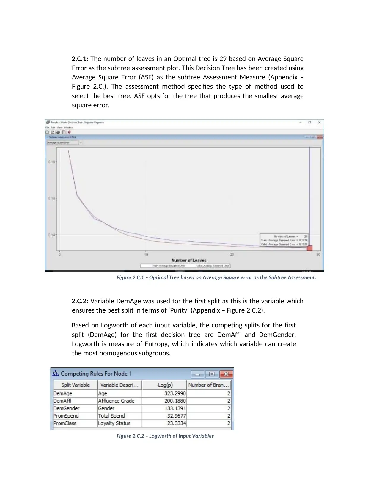
2.A: After dragging the Organics dataset to the Organics diagram, we connect
the Data Partition node to the Organics dataset. 50% of the data is utilized for
training while the remaining 50% of the data is used for validation (Appendix –
Figure 2.A). Training set is used to build a set of models while Validation set is
utilized to select the best model created from the Training set.
Figure 2.A (2) – Adding Data Partition to the Organics data source.
2.B: A Decision Tree is then connected to the Data Partition node (Appendix –
Figure 2.B)

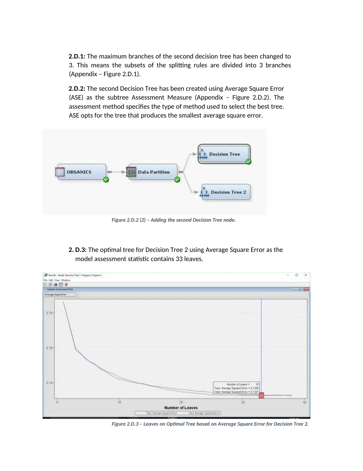
2.C.1: The number of leaves in an Optimal tree is 29 based on Average Square
Error as the subtree assessment plot. This Decision Tree has been created using
Average Square Error (ASE) as the subtree Assessment Measure (Appendix –
Figure 2.C.). The assessment method specifies the type of method used to
select the best tree. ASE opts for the tree that produces the smallest average
square error.
Figure 2.C.1 – Optimal Tree based on Average Square error as the Subtree Assessment.
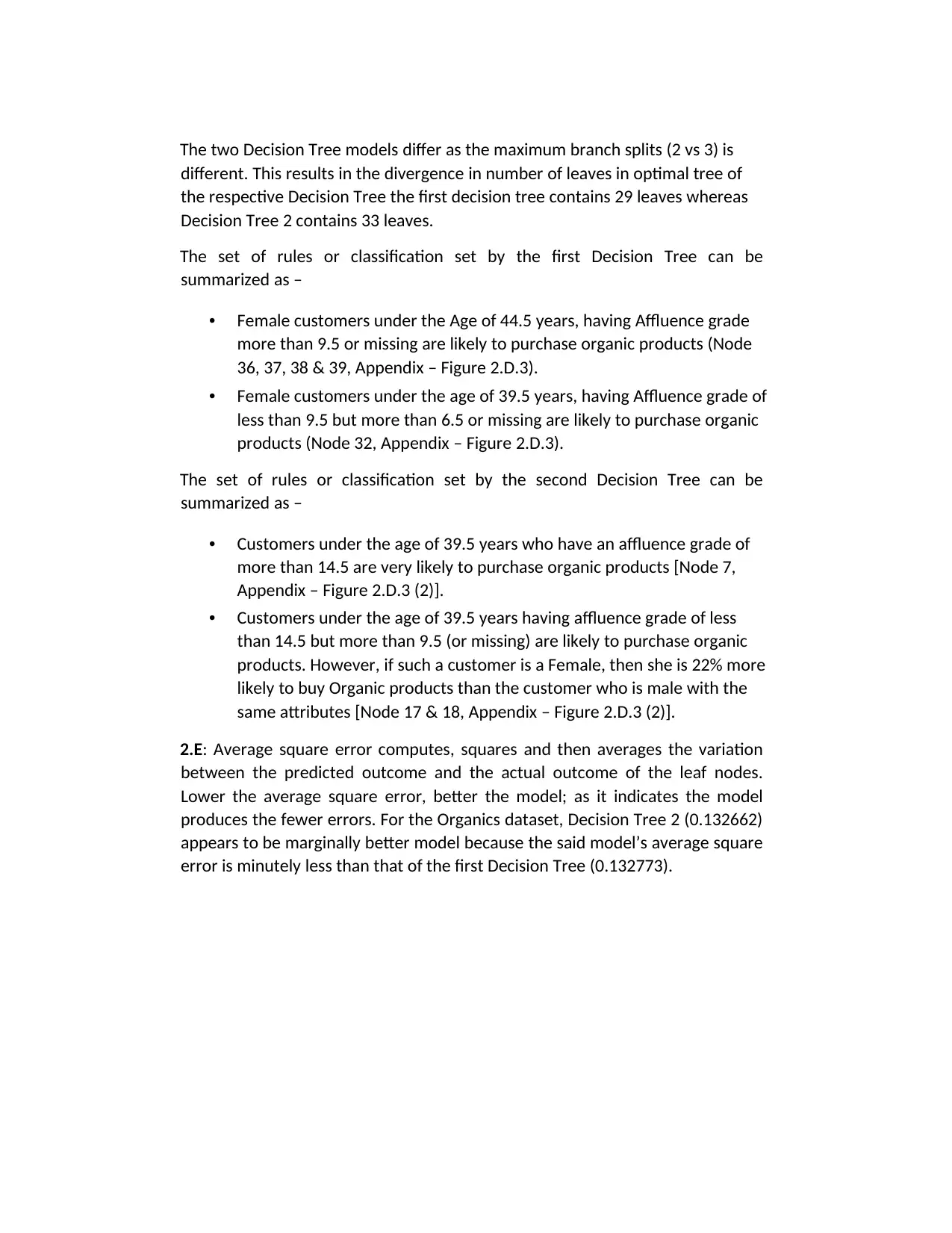
2.C.2: Variable DemAge was used for the first split as this is the variable which
ensures the best split in terms of ‘Purity’ (Appendix – Figure 2.C.2).
Based on Logworth of each input variable, the competing splits for the first
split (DemAge) for the first decision tree are DemAffl and DemGender.
Logworth is measure of Entropy, which indicates which variable can create
the most homogenous subgroups.
Figure 2.C.2 – Logworth of Input Variables

2.D.1: The maximum branches of the second decision tree has been changed to
3. This means the subsets of the splitting rules are divided into 3 branches
(Appendix – Figure 2.D.1).
2.D.2: The second Decision Tree has been created using Average Square Error
(ASE) as the subtree Assessment Measure (Appendix – Figure 2.D.2). The
assessment method specifies the type of method used to select the best tree.
ASE opts for the tree that produces the smallest average square error.
Figure 2.D.2 (2) – Adding the second Decision Tree node.
2. D.3: The optimal tree for Decision Tree 2 using Average Square Error as the
model assessment statistic contains 33 leaves.
Figure 2.D.3 – Leaves on Optimal Tree based on Average Square Error for Decision Tree 2.

The two Decision Tree models differ as the maximum branch splits (2 vs 3) is
different. This results in the divergence in number of leaves in optimal tree of
the respective Decision Tree the first decision tree contains 29 leaves whereas
Decision Tree 2 contains 33 leaves.
The set of rules or classification set by the first Decision Tree can be
summarized as –
• Female customers under the Age of 44.5 years, having Affluence grade
more than 9.5 or missing are likely to purchase organic products (Node
36, 37, 38 & 39, Appendix – Figure 2.D.3).
• Female customers under the age of 39.5 years, having Affluence grade of
less than 9.5 but more than 6.5 or missing are likely to purchase organic
products (Node 32, Appendix – Figure 2.D.3).
The set of rules or classification set by the second Decision Tree can be
summarized as –
• Customers under the age of 39.5 years who have an affluence grade of
more than 14.5 are very likely to purchase organic products [Node 7,
Appendix – Figure 2.D.3 (2)].
• Customers under the age of 39.5 years having affluence grade of less
than 14.5 but more than 9.5 (or missing) are likely to purchase organic
products. However, if such a customer is a Female, then she is 22% more
likely to buy Organic products than the customer who is male with the
same attributes [Node 17 & 18, Appendix – Figure 2.D.3 (2)].
2.E: Average square error computes, squares and then averages the variation
between the predicted outcome and the actual outcome of the leaf nodes.
Lower the average square error, better the model; as it indicates the model
produces the fewer errors. For the Organics dataset, Decision Tree 2 (0.132662)
appears to be marginally better model because the said model’s average square
error is minutely less than that of the first Decision Tree (0.132773).

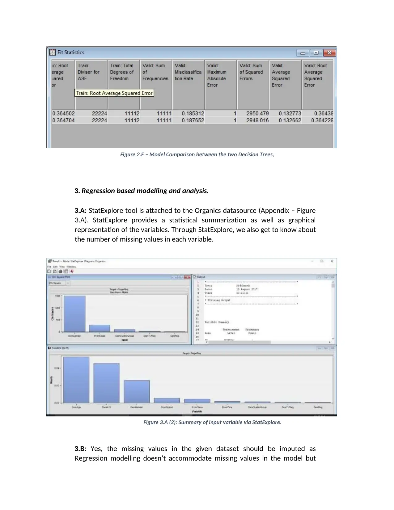
Figure 2.E – Model Comparison between the two Decision Trees,
3. Regression based modelling and analysis.
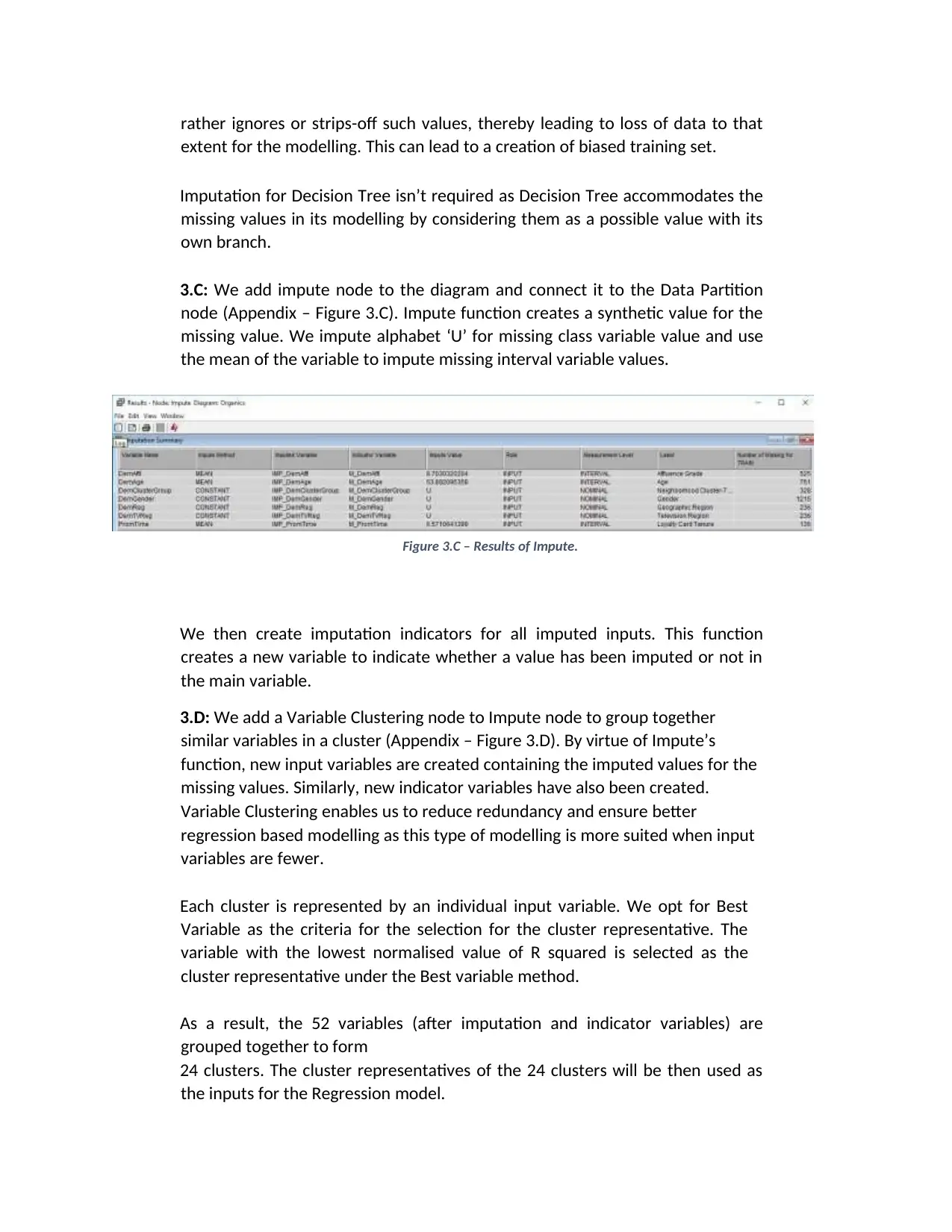
3.A: StatExplore tool is attached to the Organics datasource (Appendix – Figure
3.A). StatExplore provides a statistical summarization as well as graphical
representation of the variables. Through StatExplore, we also get to know about
the number of missing values in each variable.
Figure 3.A (2): Summary of Input variable via StatExplore.
3.B: Yes, the missing values in the given dataset should be imputed as
Regression modelling doesn’t accommodate missing values in the model but

rather ignores or strips-off such values, thereby leading to loss of data to that
extent for the modelling. This can lead to a creation of biased training set.
Imputation for Decision Tree isn’t required as Decision Tree accommodates the
missing values in its modelling by considering them as a possible value with its
own branch.
3.C: We add impute node to the diagram and connect it to the Data Partition
node (Appendix – Figure 3.C). Impute function creates a synthetic value for the
missing value. We impute alphabet ‘U’ for missing class variable value and use
the mean of the variable to impute missing interval variable values.
Figure 3.C – Results of Impute.
We then create imputation indicators for all imputed inputs. This function
creates a new variable to indicate whether a value has been imputed or not in
the main variable.
3.D: We add a Variable Clustering node to Impute node to group together
similar variables in a cluster (Appendix – Figure 3.D). By virtue of Impute’s
function, new input variables are created containing the imputed values for the
missing values. Similarly, new indicator variables have also been created.
Variable Clustering enables us to reduce redundancy and ensure better
regression based modelling as this type of modelling is more suited when input
variables are fewer.
Each cluster is represented by an individual input variable. We opt for Best
Variable as the criteria for the selection for the cluster representative. The
variable with the lowest normalised value of R squared is selected as the
cluster representative under the Best variable method.
As a result, the 52 variables (after imputation and indicator variables) are
grouped together to form
24 clusters. The cluster representatives of the 24 clusters will be then used as
the inputs for the Regression model.

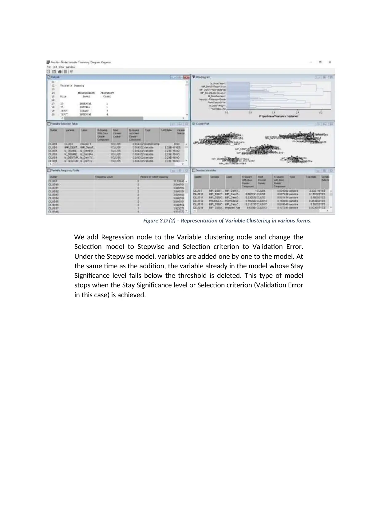
Figure 3.D (2) – Representation of Variable Clustering in various forms.
We add Regression node to the Variable clustering node and change the
Selection model to Stepwise and Selection criterion to Validation Error.
Under the Stepwise model, variables are added one by one to the model. At
the same time as the addition, the variable already in the model whose Stay
Significance level falls below the threshold is deleted. This type of model
stops when the Stay Significance level or Selection criterion (Validation Error
in this case) is achieved.

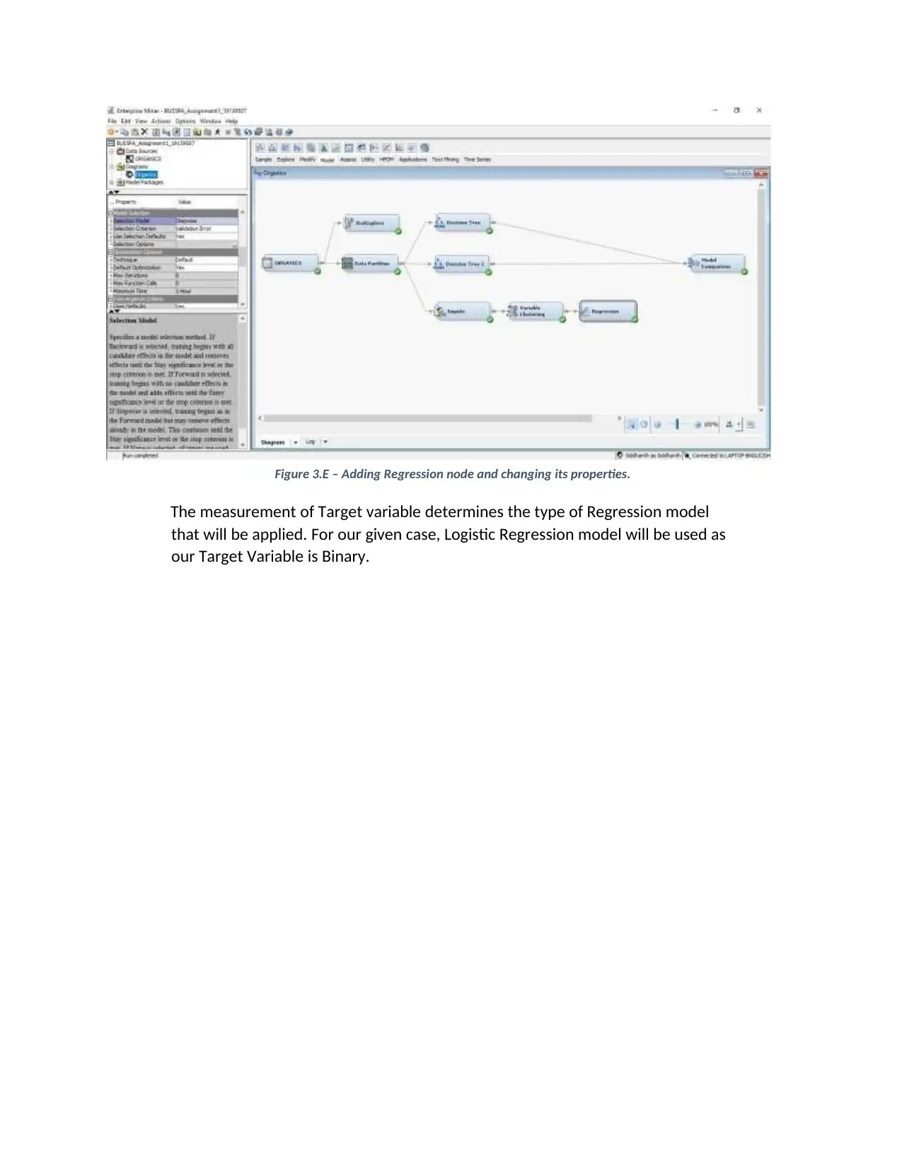
Figure 3.E – Adding Regression node and changing its properties.
The measurement of Target variable determines the type of Regression model
that will be applied. For our given case, Logistic Regression model will be used as
our Target Variable is Binary.