BUS5SBF Assignment: Household Data Analysis in Business Finance

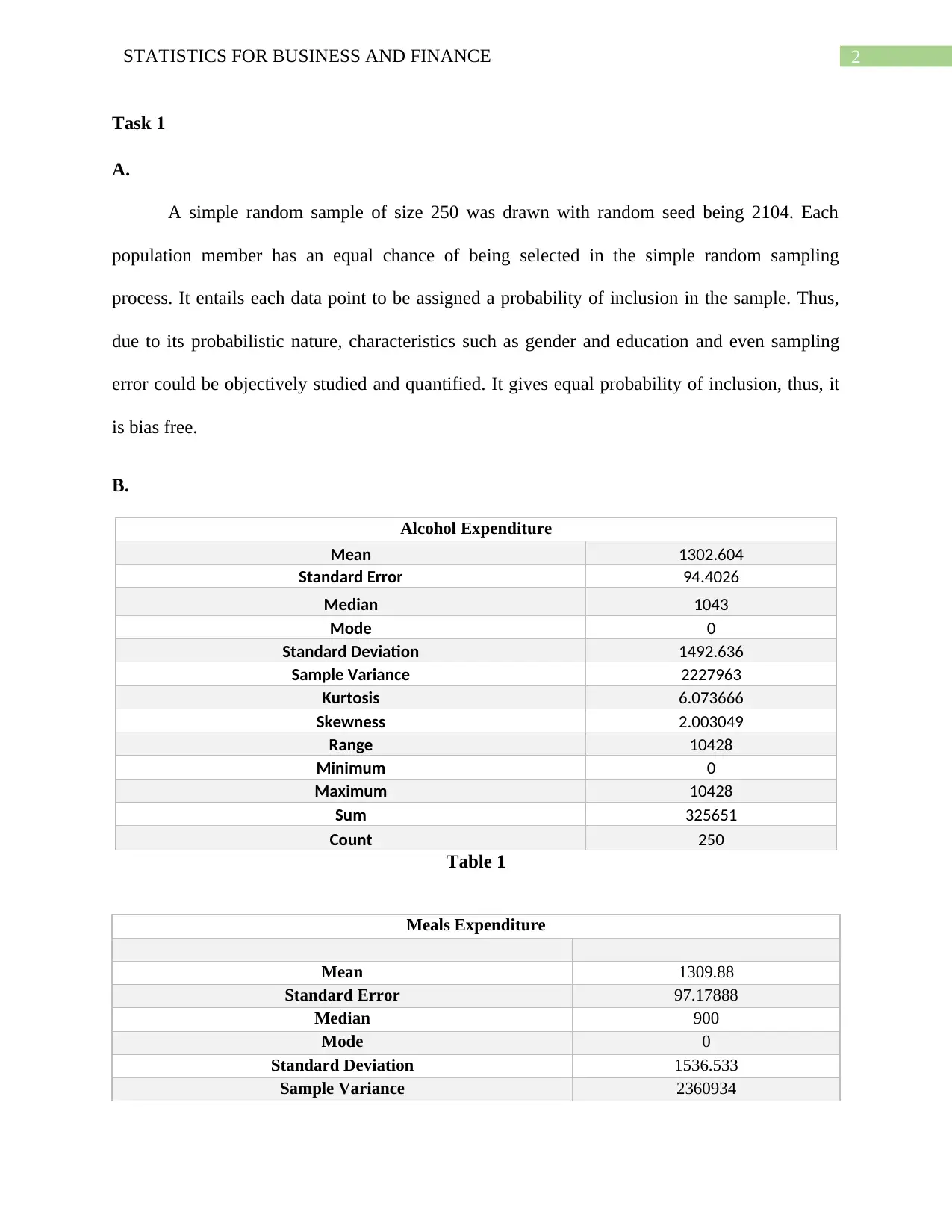
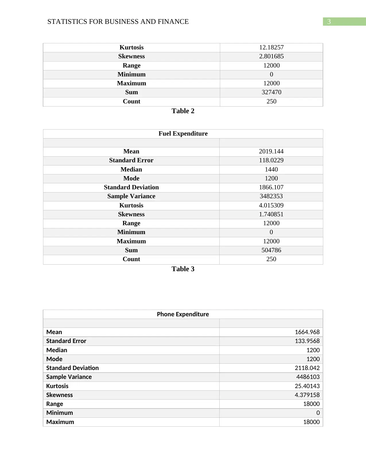
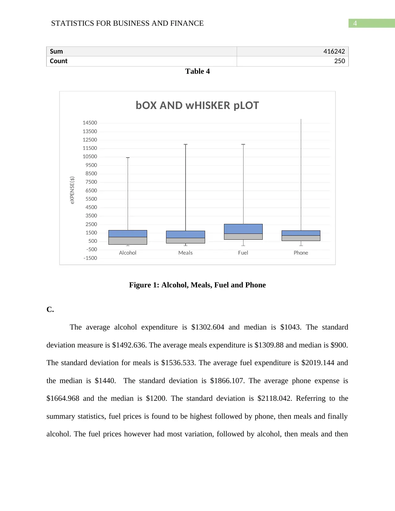
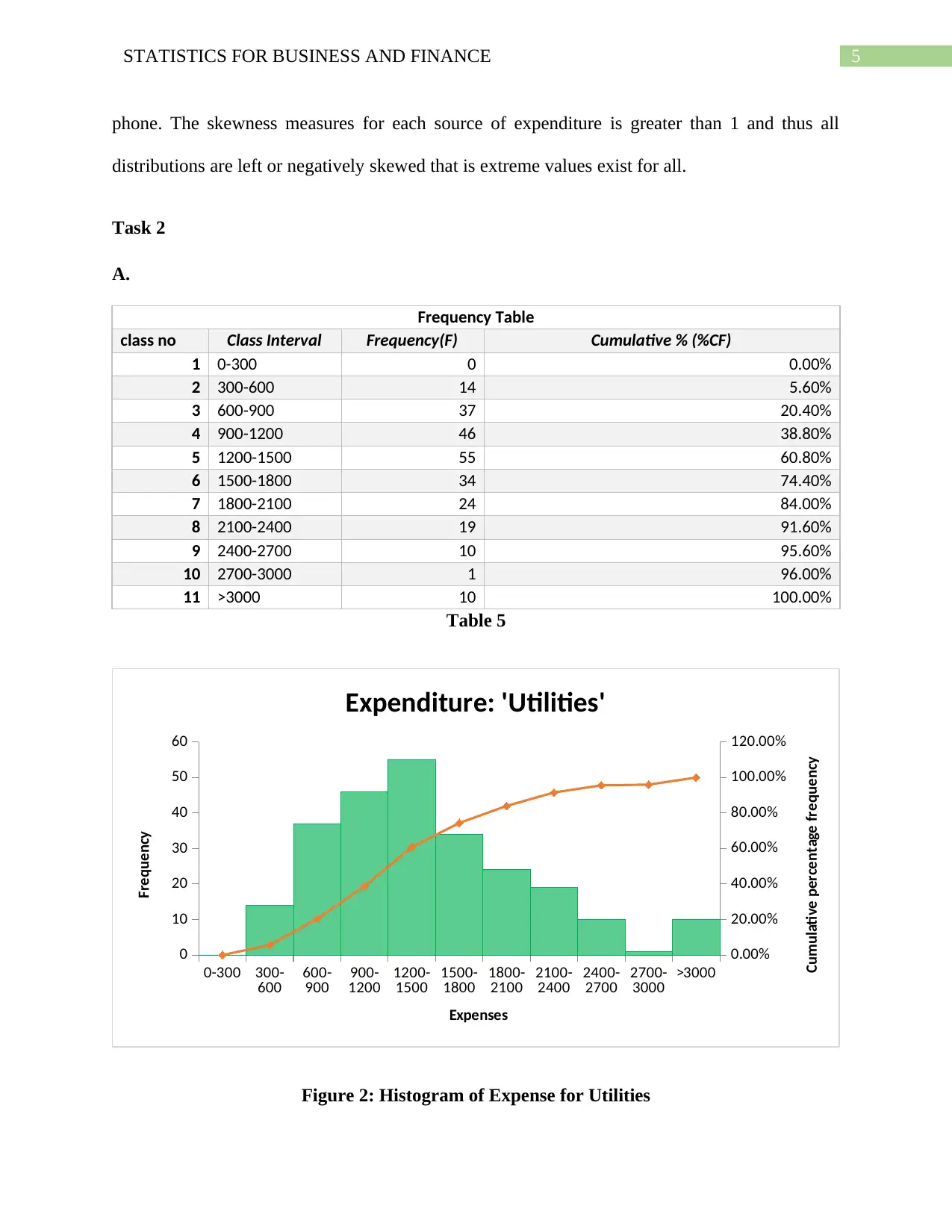
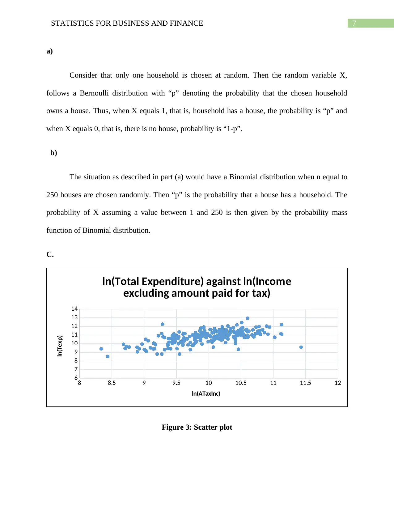
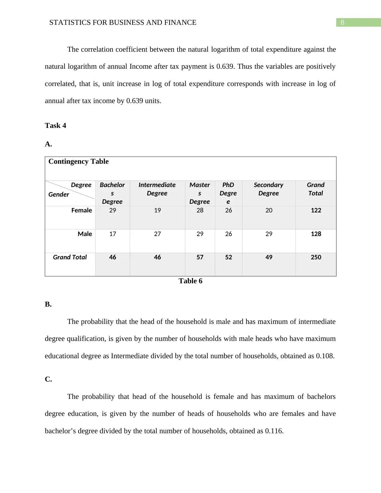
This report presents a statistical analysis of household data, covering various expenditure categories and demographic factors. The analysis includes descriptive statistics for alcohol, meals, fuel, and phone expenditures, revealing variations in averages, medians, and standard deviations. A frequency distribution and histogram are used to analyze utility expenses, determining the percentage of households spending within specific ranges. The report also identifies the top and bottom 5% of after-tax incomes and examines the correlation between total expenditure and after-tax income. A contingency table analyzes the relationship between gender and education levels, calculating probabilities related to household heads. The analysis utilizes simple random sampling with a sample size of 250 and examines the skewness of the data. This assignment solution is available on Desklib, a platform offering a range of study tools and resources for students.

Running head: STATISTICS FOR BUSINESS AND FINANCE
Statistics for Business and Finance
Name of Student
Name of University
Author Note

1STATISTICS FOR BUSINESS AND FINANCE
Table of Contents
Task 1...............................................................................................................................................3
A..................................................................................................................................................3
B...................................................................................................................................................3
C...................................................................................................................................................5
Task 2...............................................................................................................................................6
A..................................................................................................................................................6
B...................................................................................................................................................7
Task 3...............................................................................................................................................7
A..................................................................................................................................................7
B...................................................................................................................................................7
C...................................................................................................................................................8
Task 4...............................................................................................................................................9
A..................................................................................................................................................9
B...................................................................................................................................................9
C...................................................................................................................................................9
D................................................................................................................................................10
E.................................................................................................................................................10

2STATISTICS FOR BUSINESS AND FINANCE
Task 1
A.
A simple random sample of size 250 was drawn with random seed being 2104. Each
population member has an equal chance of being selected in the simple random sampling
process. It entails each data point to be assigned a probability of inclusion in the sample. Thus,
due to its probabilistic nature, characteristics such as gender and education and even sampling
error could be objectively studied and quantified. It gives equal probability of inclusion, thus, it
is bias free.
B.
Alcohol Expenditure
Mean 1302.604
Standard Error 94.4026
Median 1043
Mode 0
Standard Deviation 1492.636
Sample Variance 2227963
Kurtosis 6.073666
Skewness 2.003049
Range 10428
Minimum 0
Maximum 10428
Sum 325651
Count 250
Table 1
Meals Expenditure
Mean 1309.88
Standard Error 97.17888
Median 900
Mode 0
Standard Deviation 1536.533
Sample Variance 2360934

3STATISTICS FOR BUSINESS AND FINANCE
Kurtosis 12.18257
Skewness 2.801685
Range 12000
Minimum 0
Maximum 12000
Sum 327470
Count 250
Table 2
Fuel Expenditure
Mean 2019.144
Standard Error 118.0229
Median 1440
Mode 1200
Standard Deviation 1866.107
Sample Variance 3482353
Kurtosis 4.015309
Skewness 1.740851
Range 12000
Minimum 0
Maximum 12000
Sum 504786
Count 250
Table 3
Phone Expenditure
Mean 1664.968
Standard Error 133.9568
Median 1200
Mode 1200
Standard Deviation 2118.042
Sample Variance 4486103
Kurtosis 25.40143
Skewness 4.379158
Range 18000
Minimum 0
Maximum 18000

4STATISTICS FOR BUSINESS AND FINANCE
Sum 416242
Count 250
Table 4
Alcohol Meals Fuel Phone
-1500
-500
500
1500
2500
3500
4500
5500
6500
7500
8500
9500
10500
11500
12500
13500
14500
bOX AND wHISKER pLOT
eXPENSE($)
Figure 1: Alcohol, Meals, Fuel and Phone
C.
The average alcohol expenditure is $1302.604 and median is $1043. The standard
deviation measure is $1492.636. The average meals expenditure is $1309.88 and median is $900.
The standard deviation for meals is $1536.533. The average fuel expenditure is $2019.144 and
the median is $1440. The standard deviation is $1866.107. The average phone expense is
$1664.968 and the median is $1200. The standard deviation is $2118.042. Referring to the
summary statistics, fuel prices is found to be highest followed by phone, then meals and finally
alcohol. The fuel prices however had most variation, followed by alcohol, then meals and then

5STATISTICS FOR BUSINESS AND FINANCE
phone. The skewness measures for each source of expenditure is greater than 1 and thus all
distributions are left or negatively skewed that is extreme values exist for all.
Task 2
A.
Frequency Table
class no Class Interval Frequency(F) Cumulative % (%CF)
1 0-300 0 0.00%
2 300-600 14 5.60%
3 600-900 37 20.40%
4 900-1200 46 38.80%
5 1200-1500 55 60.80%
6 1500-1800 34 74.40%
7 1800-2100 24 84.00%
8 2100-2400 19 91.60%
9 2400-2700 10 95.60%
10 2700-3000 1 96.00%
11 >3000 10 100.00%
Table 5
0-300 300-
600 600-
900 900-
1200 1200-
1500 1500-
1800 1800-
2100 2100-
2400 2400-
2700 2700-
3000 >3000
0
10
20
30
40
50
60
0.00%
20.00%
40.00%
60.00%
80.00%
100.00%
120.00%
Expenditure: 'Utilities'
Expenses
Frequency
Cumulative percentage frequency
Figure 2: Histogram of Expense for Utilities

6STATISTICS FOR BUSINESS AND FINANCE
B.
a)
Percentage of households found to be spending at most $900 per annum on utilities is
20.40%.
b)
Percentage of households found to be spending at between $1500 and $2700 per annum
on utilities is 34.8%.
c)
Percentage of households found to be spending more than $3000 on utilities is 4%.
Task 3
A.
The top 5% value of annual after tax income (AtaxInc) of the households is $143023.30
and the bottom 5% value is $12148.5.
The top 5% value of the dataset implies the 95th percentile value of the data. The bottom
5% value similarly implies the 5th percentile value of the data.
B.
i)
The number of households which have houses, denoted by X, measure count of
household which own a house and is therefore a quantitative variable.
ii)

7STATISTICS FOR BUSINESS AND FINANCE
a)
Consider that only one household is chosen at random. Then the random variable X,
follows a Bernoulli distribution with “p” denoting the probability that the chosen household
owns a house. Thus, when X equals 1, that is, household has a house, the probability is “p” and
when X equals 0, that is, there is no house, probability is “1-p”.
b)
The situation as described in part (a) would have a Binomial distribution when n equal to
250 houses are chosen randomly. Then “p” is the probability that a house has a household. The
probability of X assuming a value between 1 and 250 is then given by the probability mass
function of Binomial distribution.
C.
8 8.5 9 9.5 10 10.5 11 11.5 12
6
7
8
9
10
11
12
13
14
ln(Total Expenditure) against ln(Income
excluding amount paid for tax)
ln(ATaxInc)
ln(Texp)
Figure 3: Scatter plot

8STATISTICS FOR BUSINESS AND FINANCE
The correlation coefficient between the natural logarithm of total expenditure against the
natural logarithm of annual Income after tax payment is 0.639. Thus the variables are positively
correlated, that is, unit increase in log of total expenditure corresponds with increase in log of
annual after tax income by 0.639 units.
Task 4
A.
Contingency Table
Degree Bachelor
s
Degree
Intermediate
Degree
Master
s
Degree
PhD
Degre
e
Secondary
Degree
Grand
TotalGender
Female 29 19 28 26 20 122
Male 17 27 29 26 29 128
Grand Total 46 46 57 52 49 250
Table 6
B.
The probability that the head of the household is male and has maximum of intermediate
degree qualification, is given by the number of households with male heads who have maximum
educational degree as Intermediate divided by the total number of households, obtained as 0.108.
C.
The probability that head of the household is female and has maximum of bachelors
degree education, is given by the number of heads of households who are females and have
bachelor’s degree divided by the total number of households, obtained as 0.116.

9STATISTICS FOR BUSINESS AND FINANCE
D.
The proportion of male household heads with secondary degree as highest education
degree is given by the number of male household heads with secondary education divided by
total number of male household heads, obtained as 0.2266.
E.
The probability of “head of household is female” is 0.488 and the probability of “has a
master’s degree” is 0.228. The product of the events is computed to be 0.111. Again, the
probability of their union, “female head and has master’s degree” is 0.112. Therefore the
intersection is 0.001. Hence the events are not independent.