University Household Data Analysis Report - BUS5SBF Module

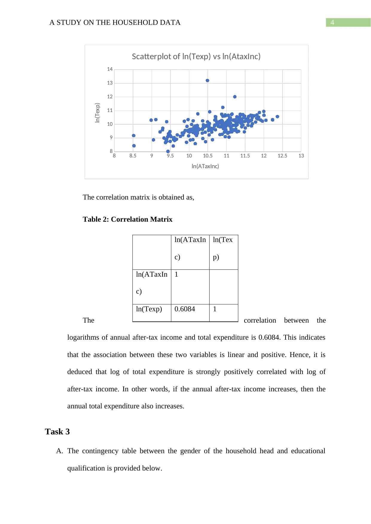
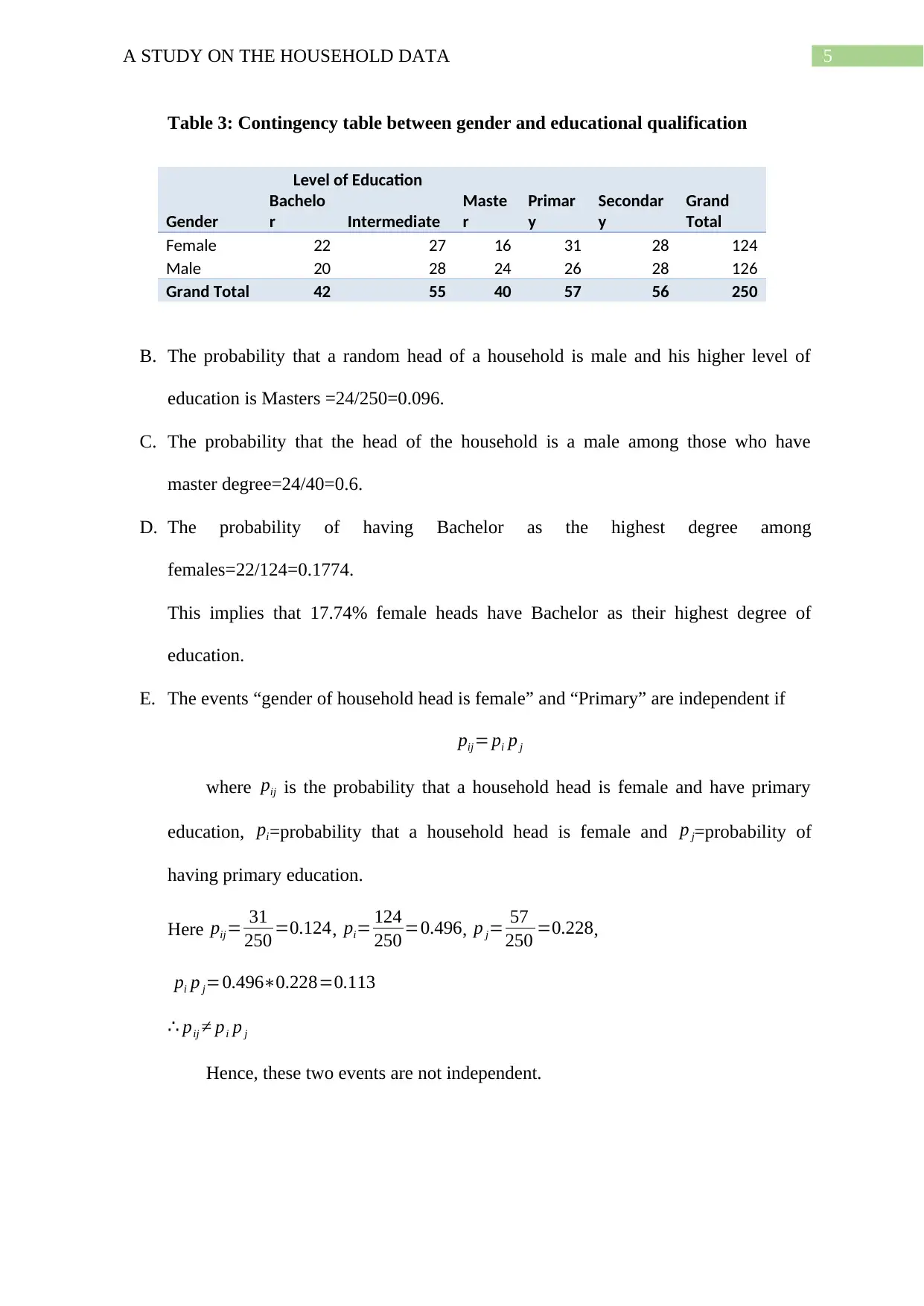
This report presents a statistical analysis of household data, focusing on income, expenditure, and related variables. The study begins with a random sample of 250 households, employing descriptive statistics and box plots to examine annual expenditures on alcohol, meals, fuel, and phones. The analysis includes measures of central tendency, dispersion, and skewness, revealing insights into spending patterns. The report then delves into after-tax income, identifying outliers and proportions related to homeownership. Using a binomial distribution, the probability of homeownership within a randomly selected group is calculated. Furthermore, a scatterplot and correlation matrix explore the relationship between after-tax income and total expenditure. Finally, the report examines the relationship between household head's gender and educational qualifications using contingency tables, calculating probabilities and assessing the independence of events.

Running Head: A STUDY ON THE HOUSEHOLD DATA
A STUDY ON THE HOUSEHOLD DATA
Name of the Student:
Name of the University:
.
Author Note:

1A STUDY ON THE HOUSEHOLD DATA
Task 1
A. Here a random sample of 250 households has been taken by using random selection
procedure. In this process, random numbers are created and the dataset is sorted
according to the generated random numbers from which the sample was selected. Due
to randomization, the sample reflects the entire population and reduces sampling
error. Moreover, all the households have equal chance of being selected in the sample.
Hence, this is the best sampling method for this data.
B. The descriptive statistics and box plots of the variables- alcohol, meals, fuel and
phone are given below.
Table 1: Descriptive Statistics
Alcohol Meals
Mean 1070.776 Mean 1105.576
Standard Error 84.6086 Standard Error 76.3080
Median 587 Median 720
Mode 0 Mode 0
Standard Deviation 1337.7795 Standard Deviation 1206.5356
Sample Variance 1789654 Sample Variance 1455728
Kurtosis 10.1459 Kurtosis 6.1005
Skewness 2.4116 Skewness 2.1274
Range 10428 Range 7800
Minimum 0 Minimum 0
Maximum 10428 Maximum 7800
Sum 267694 Sum 276394
Count 250 Count 250
Fuel Phone
Mean 1808.064 Mean 1392.792
Standard Error 100.3622 Standard Error 89.7956
Median 1440 Median 1080
Mode 0 Mode 1200
Standard Deviation 1586.8652 Standard Deviation 1419.7933
Sample Variance 2518141 Sample Variance 2015813
Kurtosis 3.9027 Kurtosis 17.8801
Skewness 1.5562 Skewness 3.6312
Range 10200 Range 10800
Minimum 0 Minimum 0
Maximum 10200 Maximum 10800

2A STUDY ON THE HOUSEHOLD DATA
Sum 452016 Sum 348198
Count 250 Count 250
Graph 1: Boxplots for expenditures
C. Table 1 shows that on average, the annual expenditures on alcohol, meals, fuel and
phones are 1070.7761071, 1105.5761106, 1808.0641808 and 1392.7921393
AUD respectively. The standard deviations are 1337.7795, 1206.5356, 1586.8652 and
1419.7933 respectively, which indicate that the data points are widely varied. The
median shows that in 50% households, the annual expenditure on alcohol is less than
587AUD. 50% household spent less than 720 AUD on meals, 740 AUD on fuel and
less than 1080AUD on phone annually. The minimum value for any of these
expenditure is 0. The mean is greater than the median in each case. Moreover, the
skewness coefficients are also positive. Hence, the distributions of annual expenditure
of each of the mentioned variables are positively skewed.
The graph shows that the medians are closer to the first quartile than the third
quartile for each of the variables. This implies that the distribution is positively

3A STUDY ON THE HOUSEHOLD DATA
skewed for each variable. Further, it can be observed that the variable fuel has least
number of outliers and phone has highest number of outliers. Hence, it can be
concluded that there are too many cases where the annual expenditures on phone is
unexpectedly high. Comparatively, there are a smaller number of cases where the
annual expenditure is unexpectedly high, for rest of the variables.
Task 2
A. From the information on annual after-tax income, it can be observed that there are
10% cases that have AtaxInc less than 14521.814522 AUD or have AtaxInc greater
than 106789.5106790 AUD. Further, it has been noted that there are 25 households
which have annual after tax-income less than 14522 AUD and 25 have greater than
106790 AUD.
B. Here OwnHouse is a categorical variable indicating 1 for a household that owns house
and 0 otherwise. The proportion of households who owns house is obtained as 0.752
that is around 75% households have their own home.
The variable has only two outcome 0 and 1 and probability of success is given.
Hence, a binomial distribution can be formed as Bin (n, p) where n=5, p=0.752.
∴ P ( X=3 ) = C3
5 ( 0.752 )3 (1−0.752 )5−3=0.2615
Therefore, the probability that any three of the five randomly chosen households will
own a house is 0.2615.
C. The scatterplot for ln(Texp) against ln(ATaxInc) is given below.
Graph 2: Scatterplot

4A STUDY ON THE HOUSEHOLD DATA
8 8.5 9 9.5 10 10.5 11 11.5 12 12.5 13
8
9
10
11
12
13
14
Scatterplot of ln(Texp) vs ln(AtaxInc)
ln(ATaxInc)
ln(Texp)
The correlation matrix is obtained as,
Table 2: Correlation Matrix
The correlation between the
logarithms of annual after-tax income and total expenditure is 0.6084. This indicates
that the association between these two variables is linear and positive. Hence, it is
deduced that log of total expenditure is strongly positively correlated with log of
after-tax income. In other words, if the annual after-tax income increases, then the
annual total expenditure also increases.
Task 3
A. The contingency table between the gender of the household head and educational
qualification is provided below.
ln(ATaxIn
c)
ln(Tex
p)
ln(ATaxIn
c)
1
ln(Texp) 0.6084 1

5A STUDY ON THE HOUSEHOLD DATA
Table 3: Contingency table between gender and educational qualification
Level of Education
Gender
Bachelo
r Intermediate
Maste
r
Primar
y
Secondar
y
Grand
Total
Female 22 27 16 31 28 124
Male 20 28 24 26 28 126
Grand Total 42 55 40 57 56 250
B. The probability that a random head of a household is male and his higher level of
education is Masters =24/250=0.096.
C. The probability that the head of the household is a male among those who have
master degree=24/40=0.6.
D. The probability of having Bachelor as the highest degree among
females=22/124=0.1774.
This implies that 17.74% female heads have Bachelor as their highest degree of
education.
E. The events “gender of household head is female” and “Primary” are independent if
pij= pi p j
where pij is the probability that a household head is female and have primary
education, pi=probability that a household head is female and p j=probability of
having primary education.
Here pij= 31
250 =0.124, pi= 124
250 =0.496, p j= 57
250 =0.228,
pi p j=0.496∗0.228=0.113
∴ pij ≠ pi p j
Hence, these two events are not independent.

6A STUDY ON THE HOUSEHOLD DATA
Bibliography
Goos, P. and Meintrup, D., 2015. Statistics with JMP: graphs, descriptive statistics and
probability. John Wiley & Sons.
Johnson, D.E., 2014. 14 Descriptive statistics. Research methods in linguistics, p.288.
Winston, W., 2016. Microsoft Excel data analysis and business modeling. Microsoft press.