BUS5SBF - Statistical Analysis of Household Expenditure and Income

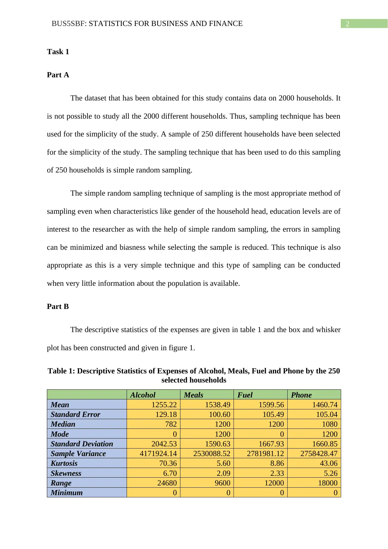
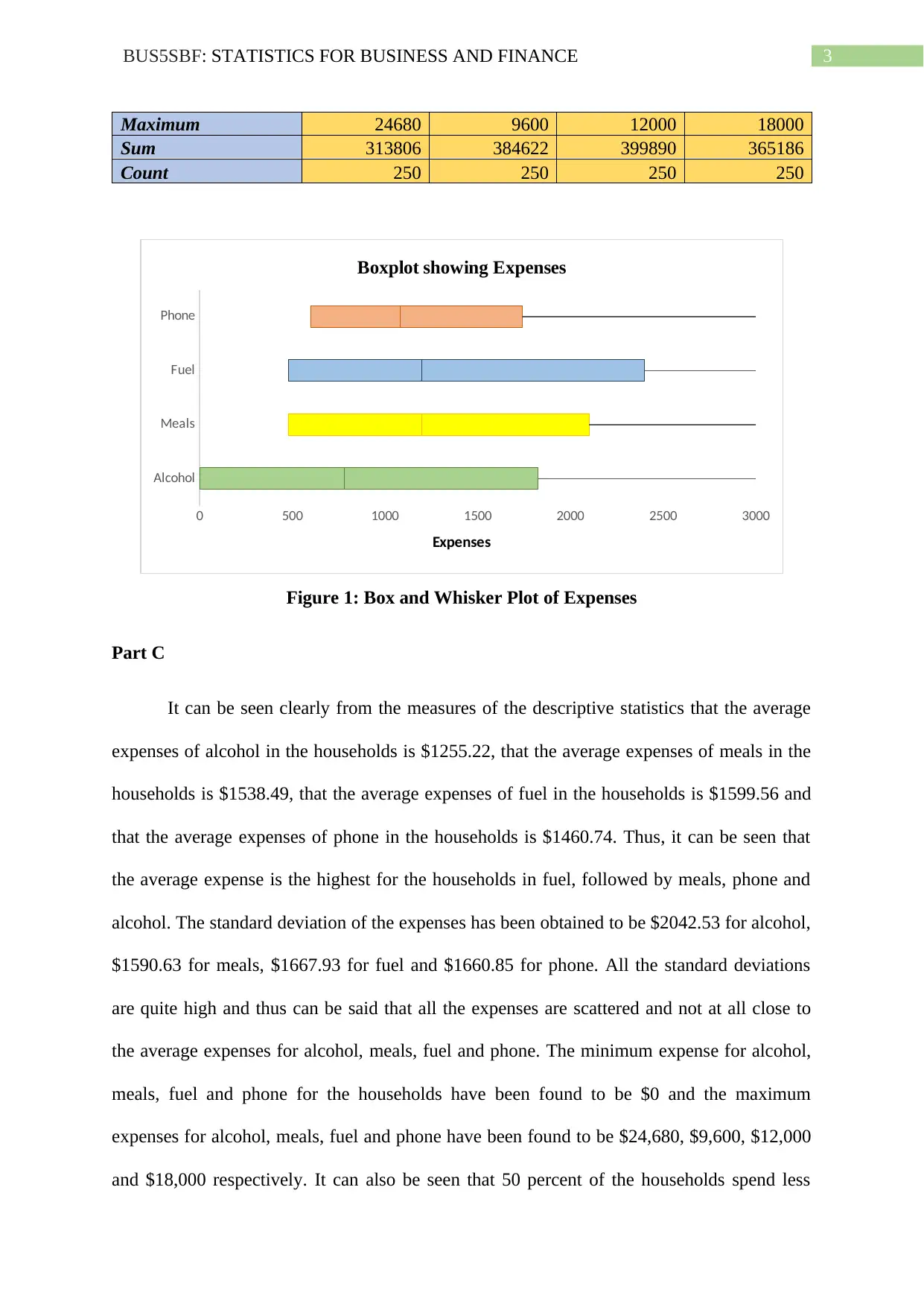
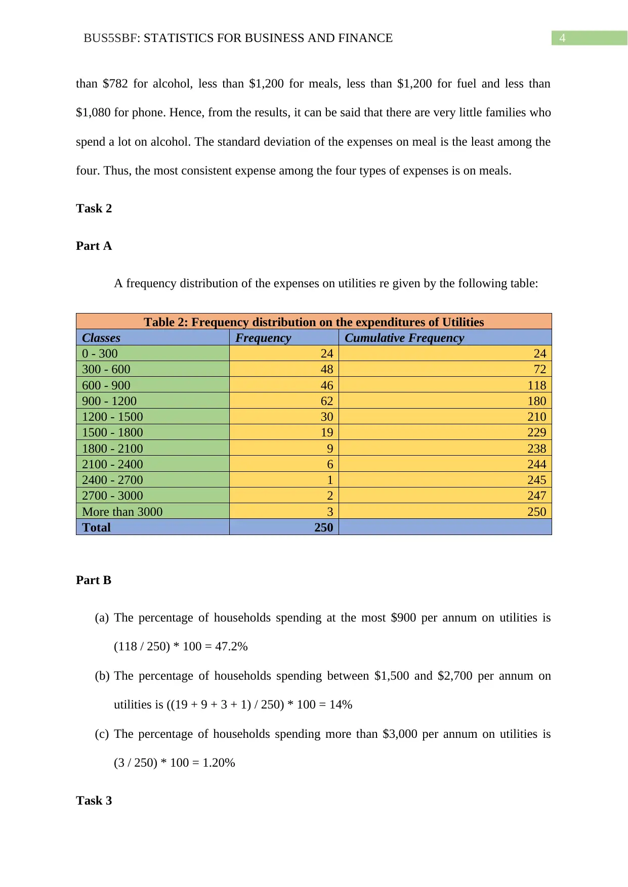
This report presents a statistical analysis of household financial data, utilizing a sample of 250 households selected via simple random sampling from a dataset of 2000 households. The analysis includes descriptive statistics of expenses on alcohol, meals, fuel, and phone, revealing that fuel has t...Read More

Running Head: BUS5SBF: STATISTICS FOR BUSINESS AND FINANCE
BUS5SBF: Statistics for Business and Finance
Name of the Student
Name of the University
Author Note

1BUS5SBF: STATISTICS FOR BUSINESS AND FINANCE
Table of Contents
Task 1.........................................................................................................................................2
Part A.....................................................................................................................................2
Part B......................................................................................................................................2
Part C......................................................................................................................................3
Task 2.........................................................................................................................................4
Part A.....................................................................................................................................4
Part B......................................................................................................................................4
Task 3.........................................................................................................................................5
Part A.....................................................................................................................................5
Part B......................................................................................................................................5
Part C......................................................................................................................................5
Task 4.........................................................................................................................................6
Part A.....................................................................................................................................6
Part B......................................................................................................................................6
Part C......................................................................................................................................6
Part D.....................................................................................................................................7
Part E......................................................................................................................................7

2BUS5SBF: STATISTICS FOR BUSINESS AND FINANCE
Task 1
Part A
The dataset that has been obtained for this study contains data on 2000 households. It
is not possible to study all the 2000 different households. Thus, sampling technique has been
used for the simplicity of the study. A sample of 250 different households have been selected
for the simplicity of the study. The sampling technique that has been used to do this sampling
of 250 households is simple random sampling.
The simple random sampling technique of sampling is the most appropriate method of
sampling even when characteristics like gender of the household head, education levels are of
interest to the researcher as with the help of simple random sampling, the errors in sampling
can be minimized and biasness while selecting the sample is reduced. This technique is also
appropriate as this is a very simple technique and this type of sampling can be conducted
when very little information about the population is available.
Part B
The descriptive statistics of the expenses are given in table 1 and the box and whisker
plot has been constructed and given in figure 1.
Table 1: Descriptive Statistics of Expenses of Alcohol, Meals, Fuel and Phone by the 250
selected households
Alcohol Meals Fuel Phone
Mean 1255.22 1538.49 1599.56 1460.74
Standard Error 129.18 100.60 105.49 105.04
Median 782 1200 1200 1080
Mode 0 1200 0 1200
Standard Deviation 2042.53 1590.63 1667.93 1660.85
Sample Variance 4171924.14 2530088.52 2781981.12 2758428.47
Kurtosis 70.36 5.60 8.86 43.06
Skewness 6.70 2.09 2.33 5.26
Range 24680 9600 12000 18000
Minimum 0 0 0 0

3BUS5SBF: STATISTICS FOR BUSINESS AND FINANCE
Maximum 24680 9600 12000 18000
Sum 313806 384622 399890 365186
Count 250 250 250 250
Alcohol
Meals
Fuel
Phone
0 500 1000 1500 2000 2500 3000
Boxplot showing Expenses
Expenses
Figure 1: Box and Whisker Plot of Expenses
Part C
It can be seen clearly from the measures of the descriptive statistics that the average
expenses of alcohol in the households is $1255.22, that the average expenses of meals in the
households is $1538.49, that the average expenses of fuel in the households is $1599.56 and
that the average expenses of phone in the households is $1460.74. Thus, it can be seen that
the average expense is the highest for the households in fuel, followed by meals, phone and
alcohol. The standard deviation of the expenses has been obtained to be $2042.53 for alcohol,
$1590.63 for meals, $1667.93 for fuel and $1660.85 for phone. All the standard deviations
are quite high and thus can be said that all the expenses are scattered and not at all close to
the average expenses for alcohol, meals, fuel and phone. The minimum expense for alcohol,
meals, fuel and phone for the households have been found to be $0 and the maximum
expenses for alcohol, meals, fuel and phone have been found to be $24,680, $9,600, $12,000
and $18,000 respectively. It can also be seen that 50 percent of the households spend less

4BUS5SBF: STATISTICS FOR BUSINESS AND FINANCE
than $782 for alcohol, less than $1,200 for meals, less than $1,200 for fuel and less than
$1,080 for phone. Hence, from the results, it can be said that there are very little families who
spend a lot on alcohol. The standard deviation of the expenses on meal is the least among the
four. Thus, the most consistent expense among the four types of expenses is on meals.
Task 2
Part A
A frequency distribution of the expenses on utilities re given by the following table:
Table 2: Frequency distribution on the expenditures of Utilities
Classes Frequency Cumulative Frequency
0 - 300 24 24
300 - 600 48 72
600 - 900 46 118
900 - 1200 62 180
1200 - 1500 30 210
1500 - 1800 19 229
1800 - 2100 9 238
2100 - 2400 6 244
2400 - 2700 1 245
2700 - 3000 2 247
More than 3000 3 250
Total 250
Part B
(a) The percentage of households spending at the most $900 per annum on utilities is
(118 / 250) * 100 = 47.2%
(b) The percentage of households spending between $1,500 and $2,700 per annum on
utilities is ((19 + 9 + 3 + 1) / 250) * 100 = 14%
(c) The percentage of households spending more than $3,000 per annum on utilities is
(3 / 250) * 100 = 1.20%
Task 3

5BUS5SBF: STATISTICS FOR BUSINESS AND FINANCE
Part A
The top 5% value of the annual after tax income of a household is $152,093 and the
bottom 5% value of the annual after tax income of a household is $12,480. The top 5% value
indicates that 5% of 250 selected households have an annual after tax income above $152,093
and 5% of 250 selected households have an annual after tax income below $12,480.
Part B
(i) X is a random variable denoting the number of households owning a house. Thus, X
is a quantitative variable.
(ii) (a) The probability distribution X when only one household is chosen
randomly is given by
P ( X=x ) = ( 0.648 ) x (1−0.648)1−x , x=0 , 1
Here, 0 indicates that the household selected randomly does not own a house
and 1 indicates that the household selected randomly owns a house. 0.648 is the
proportion of houses among 250 houses, who own a house.
(b) The probability distribution X when 250 households are chosen randomly
is given by P ( X=x ) =(250
x ) ( 0.648 ) x
(1−0.648)250− x, x=0 , 1 ,2 , … , 250
Part C
The correlation coefficient between the natural logarithm of total expenditures and
annual after tax income of the 250 selected households has been found to be 0.68. This
indicates there is a strong positive relationship between annual after tax income and total
expenditures of the households. If the annual after tax income increases, the total expenditure
also increases. The relationship is shown diagrammatically with the help of a scatterplot
given in figure 2.

6BUS5SBF: STATISTICS FOR BUSINESS AND FINANCE
8.5000
9.0000
9.5000
10.0000
10.5000
11.0000
11.5000
12.0000
12.5000
13.0000
13.5000
0.0000
2.0000
4.0000
6.0000
8.0000
10.0000
12.0000
14.0000
Relationship between Total Expenditure against
After Tax Income
Natural log of after tax Income
Natural log of Total Expenditure
Figure 2: Relationship between after tax income and total expenditure
Task 4
Part A
The contingency table between gender and level of education is given in the following
table 3.
Table 3: Contingency table of Gender and Education
Highest Degree of Education Gender
Female Male Grand Total
Bachelors 18 27 45
Intermediate 34 26 60
Master 31 18 49
Primary 25 22 47
Secondary 27 22 49
Grand Total 135 115 250
Part B
The probability that the head of the household is a male and his highest level of
education is intermediate is (26 / 250) = 0.104
Part C

7BUS5SBF: STATISTICS FOR BUSINESS AND FINANCE
The probability of the head of the household is a female has the bachelor’s degree is
(18 / 250) = 0.072
Part D
The proportion of having secondary as the highest degree among males is (27 / 250) =
0.108
Part E
The probability that the gender of the household head is female is (135 / 250) = 0.54
The probability that the head of the household has master’s degree is (49 / 250) = 0.196
The probability that the head of the household is a female and has a master’s degree is (31 /
250) = 0.124 ≠ (0.54 * 0.196)
Thus, the two events “Gender of the household is a female” and “having a master’s
degree” are not independent.