BUS5SBF Statistics: Household Data Analysis for Business Finance

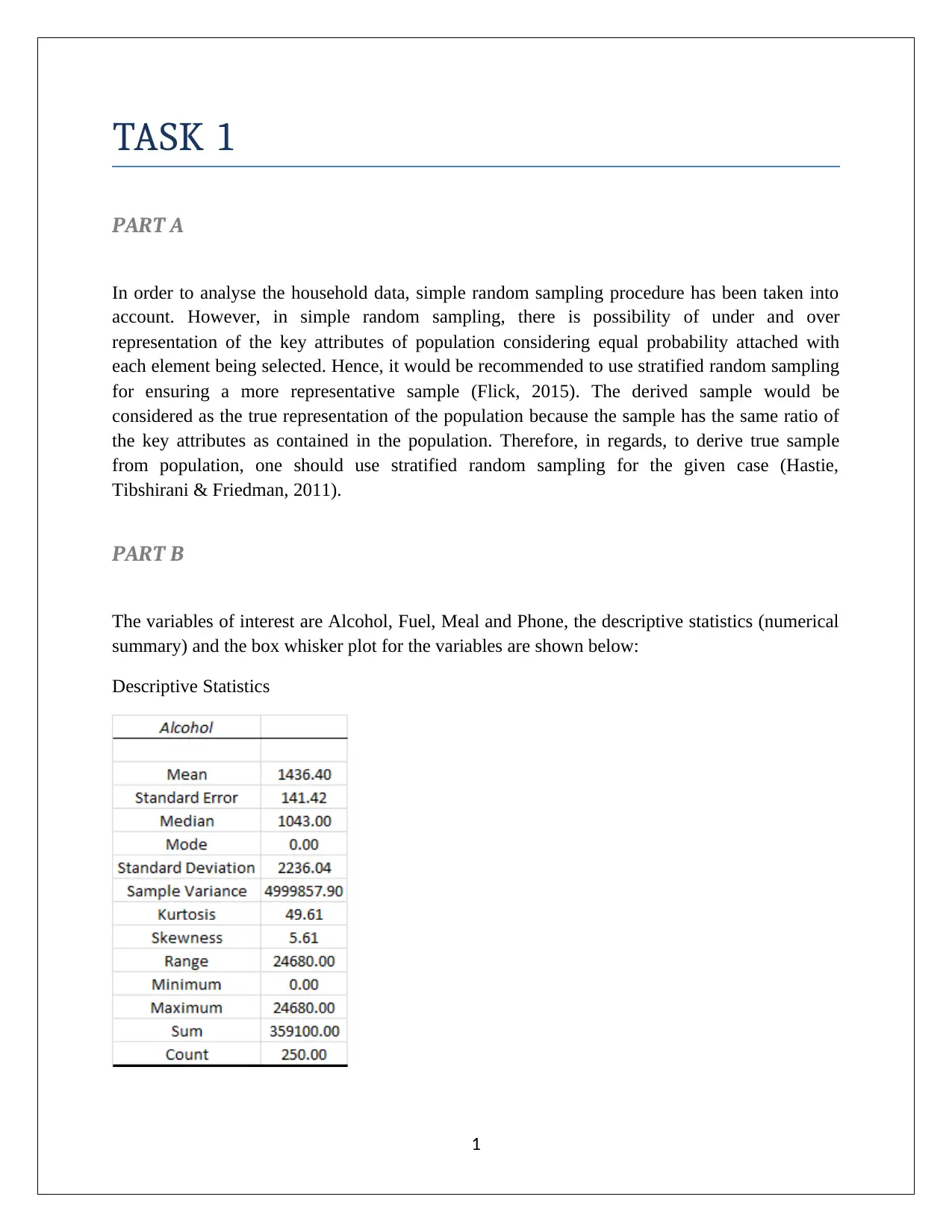
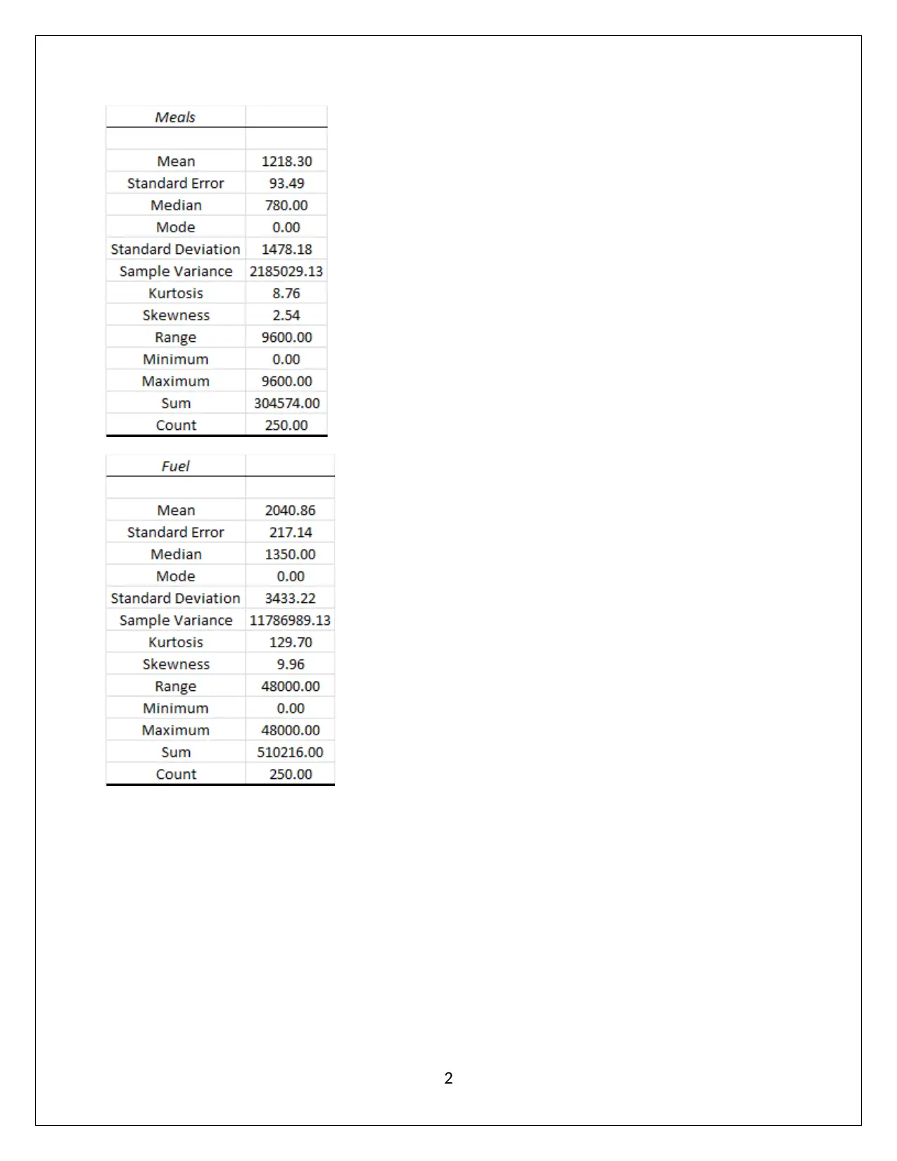
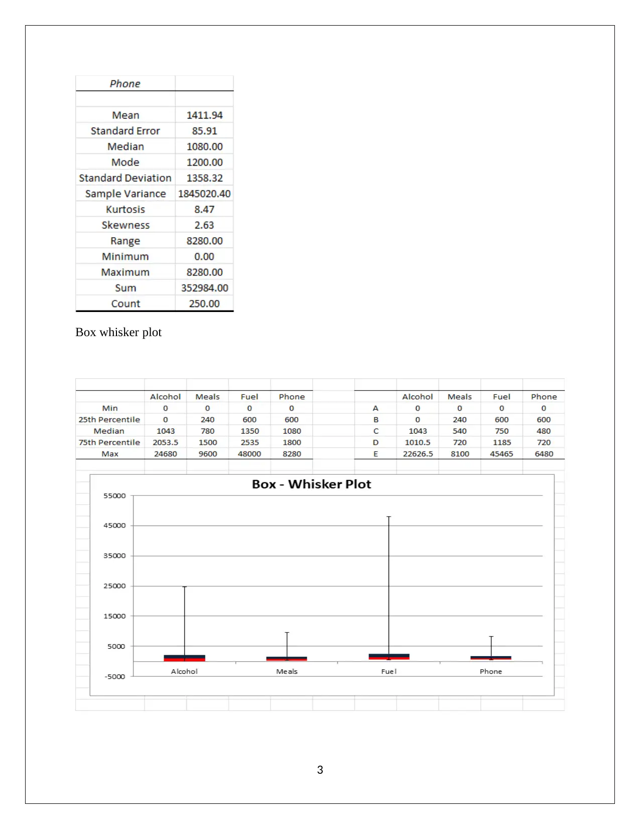
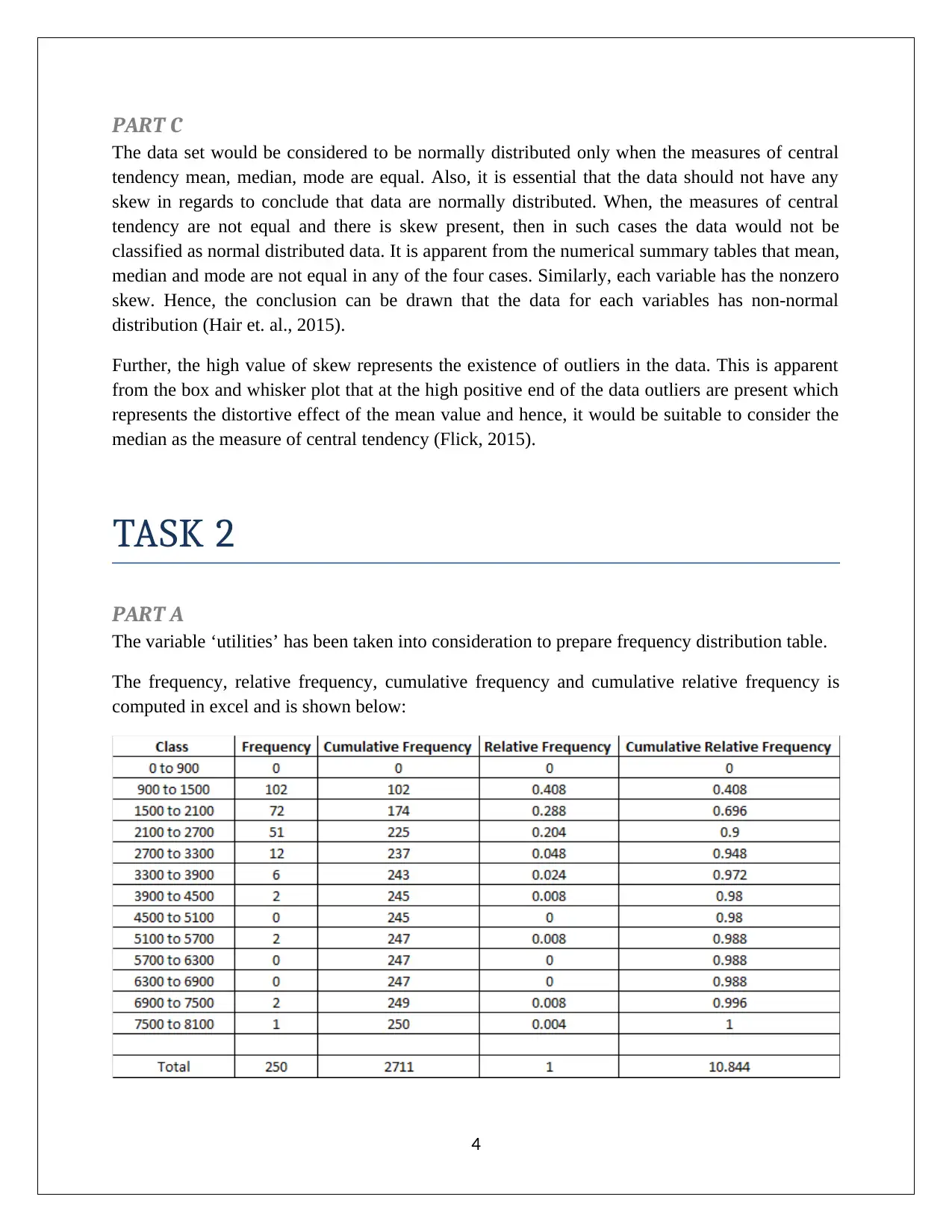
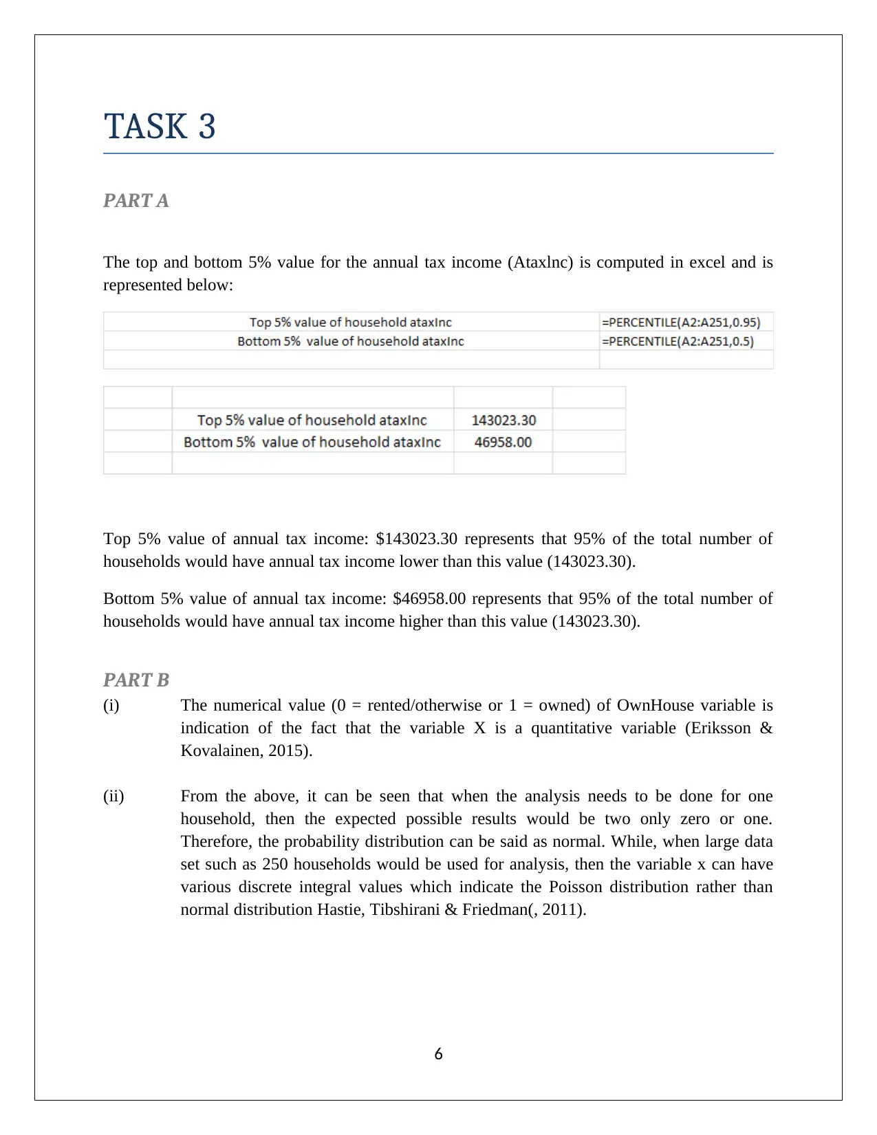
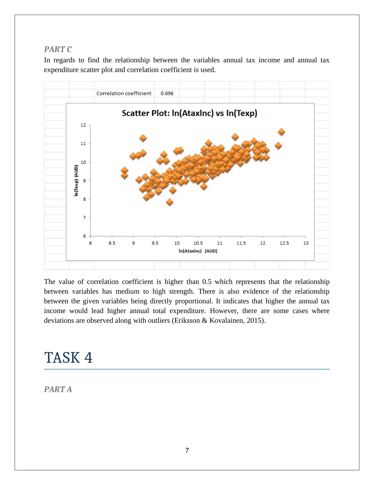
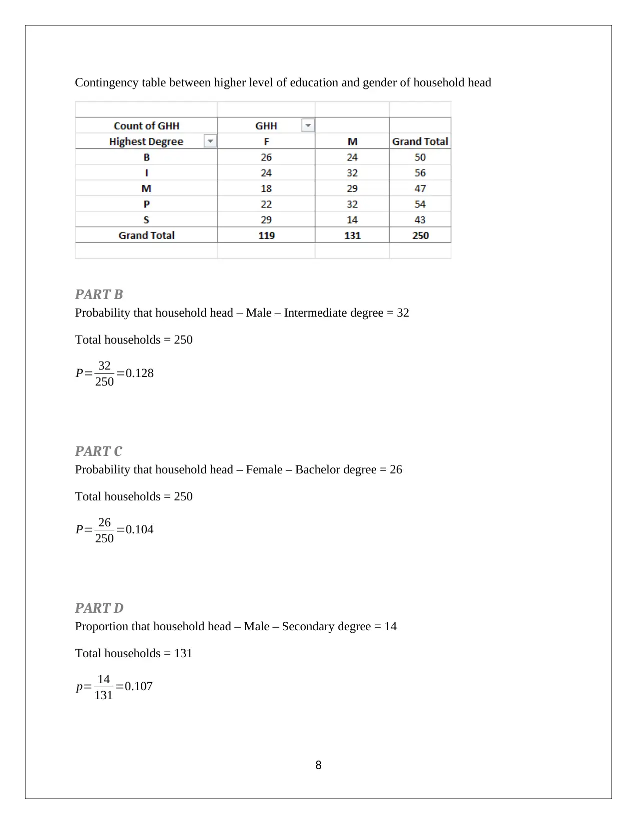
This assignment solution focuses on analyzing household data using statistical methods within the context of a Statistics for Business and Finance course (BUS5SBF). It covers various tasks including simple random sampling, stratified random sampling, descriptive statistics for variables like Alcohol, Fuel, Meal, and Phone, and normality tests. The solution also addresses frequency distribution for the 'utilities' variable, percentage calculations for household spending, and the determination of top and bottom 5% values for annual tax income. Further analysis includes exploring the relationship between annual tax income and expenditure using scatter plots and correlation coefficients, and constructing contingency tables to analyze relationships between education level and gender of household heads. The document concludes with probability calculations and independence tests, providing a comprehensive statistical analysis of the given household dataset.

Statistics For Business and Finance
Statistics For Business and Finance (BUS5SBF)
Analyzing Household Data
Student Name
[Pick the date]

TASK 1
PART A
In order to analyse the household data, simple random sampling procedure has been taken into
account. However, in simple random sampling, there is possibility of under and over
representation of the key attributes of population considering equal probability attached with
each element being selected. Hence, it would be recommended to use stratified random sampling
for ensuring a more representative sample (Flick, 2015). The derived sample would be
considered as the true representation of the population because the sample has the same ratio of
the key attributes as contained in the population. Therefore, in regards, to derive true sample
from population, one should use stratified random sampling for the given case (Hastie,
Tibshirani & Friedman, 2011).
PART B
The variables of interest are Alcohol, Fuel, Meal and Phone, the descriptive statistics (numerical
summary) and the box whisker plot for the variables are shown below:
Descriptive Statistics
1

2

Box whisker plot
3

PART C
The data set would be considered to be normally distributed only when the measures of central
tendency mean, median, mode are equal. Also, it is essential that the data should not have any
skew in regards to conclude that data are normally distributed. When, the measures of central
tendency are not equal and there is skew present, then in such cases the data would not be
classified as normal distributed data. It is apparent from the numerical summary tables that mean,
median and mode are not equal in any of the four cases. Similarly, each variable has the nonzero
skew. Hence, the conclusion can be drawn that the data for each variables has non-normal
distribution (Hair et. al., 2015).
Further, the high value of skew represents the existence of outliers in the data. This is apparent
from the box and whisker plot that at the high positive end of the data outliers are present which
represents the distortive effect of the mean value and hence, it would be suitable to consider the
median as the measure of central tendency (Flick, 2015).
TASK 2
PART A
The variable ‘utilities’ has been taken into consideration to prepare frequency distribution table.
The frequency, relative frequency, cumulative frequency and cumulative relative frequency is
computed in excel and is shown below:
4

PART B
Percentages of household hold for the given scenarios are shown below:
a. At the most of $900 per year
The given number of households heads (Sample) = 250
The number of households heads that spent on utilities at the most $ 900 per year = 0 + 102 =
102
% of households heads that spent on utilities at the most $ 900 per year =the number of
households heads that spent on utilities at the most $ 900 per year / the given number of
households heads (Sample)
= 102 / 250 = 0.408 or 40.8%
40.8% of the household would spend at most $900 per year on utilities.
b. Between $1500 per year and $2700 per year
The given number of households heads (Sample) = 250
The number of households heads that spent on utilities between $1500 per year and $2700 per
year = 72 +51 = 123
% of households heads that spent on utilities on utilities between $1500 per year and $2700 per
year = The number of households heads that spent on utilities between $1500 per year and $2700
per annum / The given number of households heads (Sample)
= 123/250 = 0.492 or 49.2 %
40.8% of the household would spend at most $900 per year on utilities.
c. More than $3000 per annum
The given number of households heads (Sample) = 250
The number of households heads that spent on utilities more than $3000 per year = 8
% of households heads that spent on utilities more than $3000 per year = The number of
households heads that spent on utilities more than $3000 per year / The given number of
households heads (Sample) = 8 / 250 = 0.032 or 3.2 %
3.20% of the household would spend more than $3000 per year on utilities.
5

TASK 3
PART A
The top and bottom 5% value for the annual tax income (Ataxlnc) is computed in excel and is
represented below:
Top 5% value of annual tax income: $143023.30 represents that 95% of the total number of
households would have annual tax income lower than this value (143023.30).
Bottom 5% value of annual tax income: $46958.00 represents that 95% of the total number of
households would have annual tax income higher than this value (143023.30).
PART B
(i) The numerical value (0 = rented/otherwise or 1 = owned) of OwnHouse variable is
indication of the fact that the variable X is a quantitative variable (Eriksson &
Kovalainen, 2015).
(ii) From the above, it can be seen that when the analysis needs to be done for one
household, then the expected possible results would be two only zero or one.
Therefore, the probability distribution can be said as normal. While, when large data
set such as 250 households would be used for analysis, then the variable x can have
various discrete integral values which indicate the Poisson distribution rather than
normal distribution Hastie, Tibshirani & Friedman(, 2011).
6

PART C
In regards to find the relationship between the variables annual tax income and annual tax
expenditure scatter plot and correlation coefficient is used.
The value of correlation coefficient is higher than 0.5 which represents that the relationship
between variables has medium to high strength. There is also evidence of the relationship
between the given variables being directly proportional. It indicates that higher the annual tax
income would lead higher annual total expenditure. However, there are some cases where
deviations are observed along with outliers (Eriksson & Kovalainen, 2015).
TASK 4
PART A
7

Contingency table between higher level of education and gender of household head
PART B
Probability that household head – Male – Intermediate degree = 32
Total households = 250
P= 32
250 =0.128
PART C
Probability that household head – Female – Bachelor degree = 26
Total households = 250
P= 26
250 =0.104
PART D
Proportion that household head – Male – Secondary degree = 14
Total households = 131
p= 14
131 =0.107
8

PART E
P ( A )=Gender as female= 119
250 =0.476
P ( B )=Having master degree= 47
250 =0.188
P ( A∧B )= 18
250 =0.072
Independent when, P ( A∧B )=P ( A ) . P ( B ) (Fehr and Grossman, 2013).
0.072 ≠ 0.476∗0.188
0.072 ≠ 0.0894
It is apparent that above condition is not satisfied and hence, the events are not said to be
independent.
9

References
Eriksson, P. & Kovalainen, A. (2015) Quantitative methods in business research (3rd ed.).
London: Sage Publications.
Fehr, F. H., & Grossman, G. (2013) An introduction to sets, probability and hypothesis testing
(3rd ed.). Ohio: Heath.
Flick, U. (2015) Introducing research methodology: A beginner's guide to doing a research
project (4th ed.). New York: Sage Publications.
Hair, J. F., Wolfinbarger, M., Money, A. H., Samouel, P., & Page, M. J. (2015) Essentials of
business research methods (2nd ed.). New York: Routledge.
Hastie, T., Tibshirani, R. & Friedman, J. (2011) The Elements of Statistical Learning (4th
ed.). New York: Springer Publications.
10