BUS5SBF Statistics for Business: Household Data Analysis Report

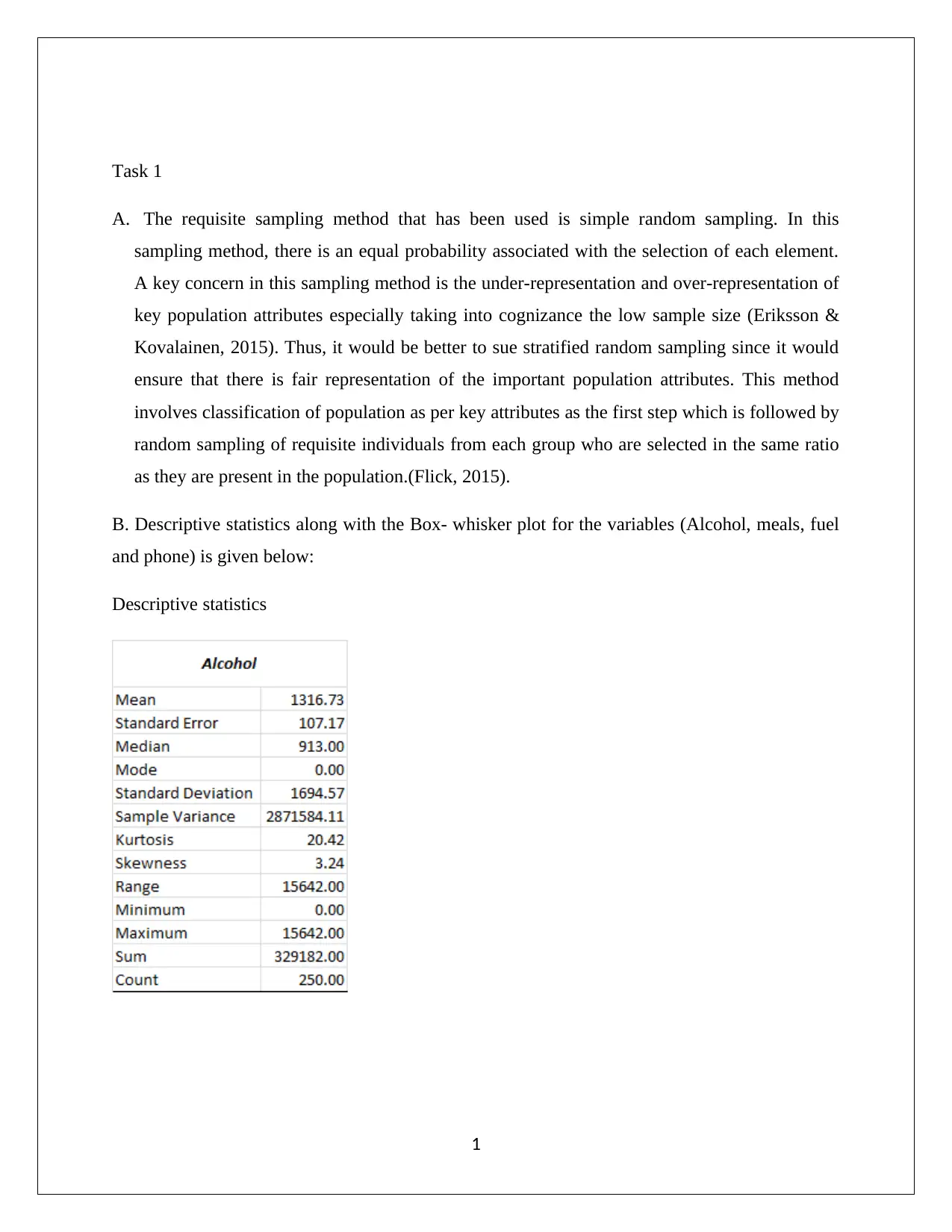
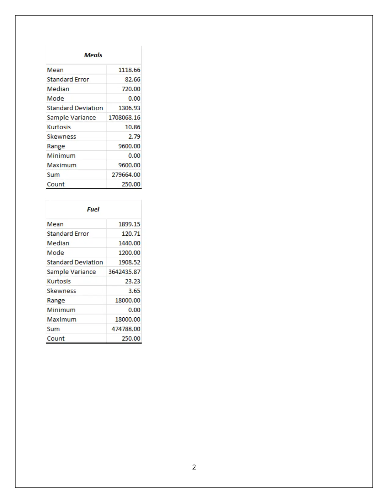
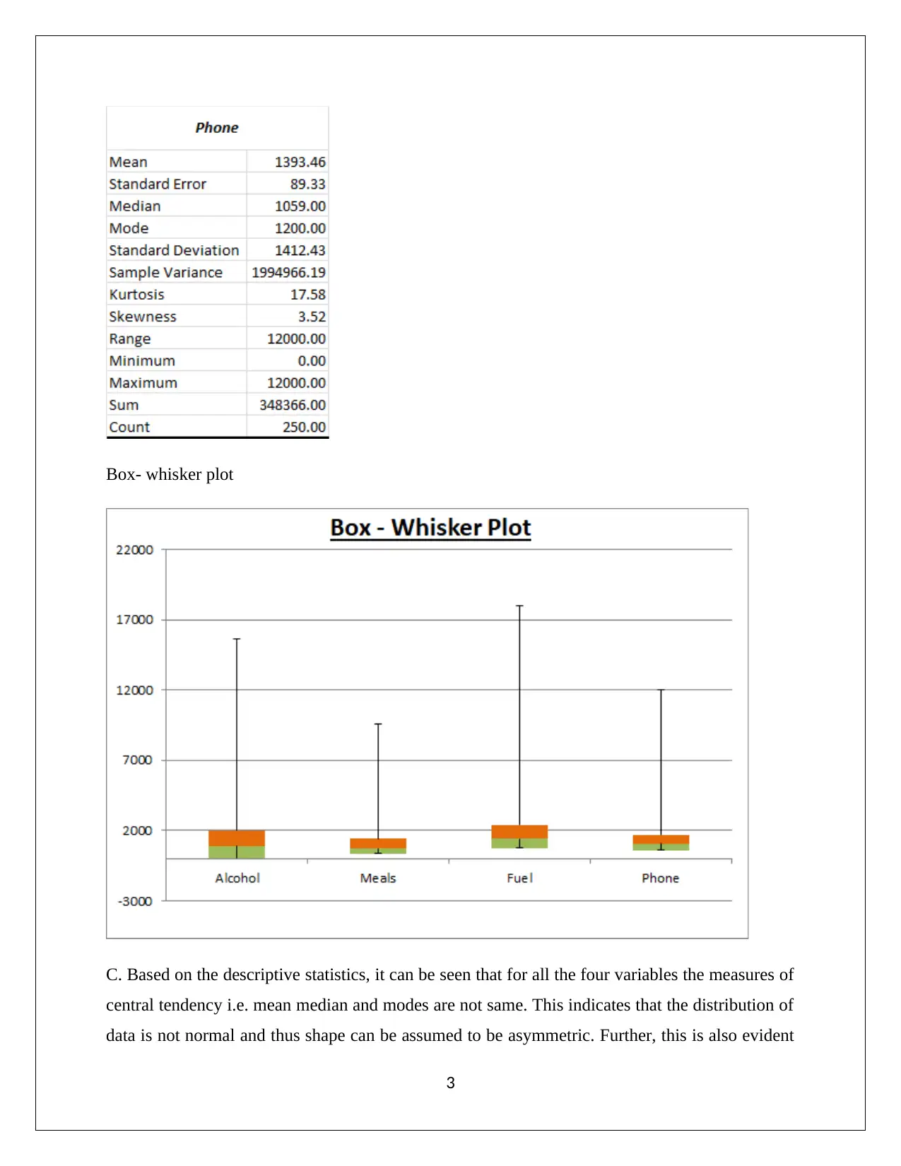
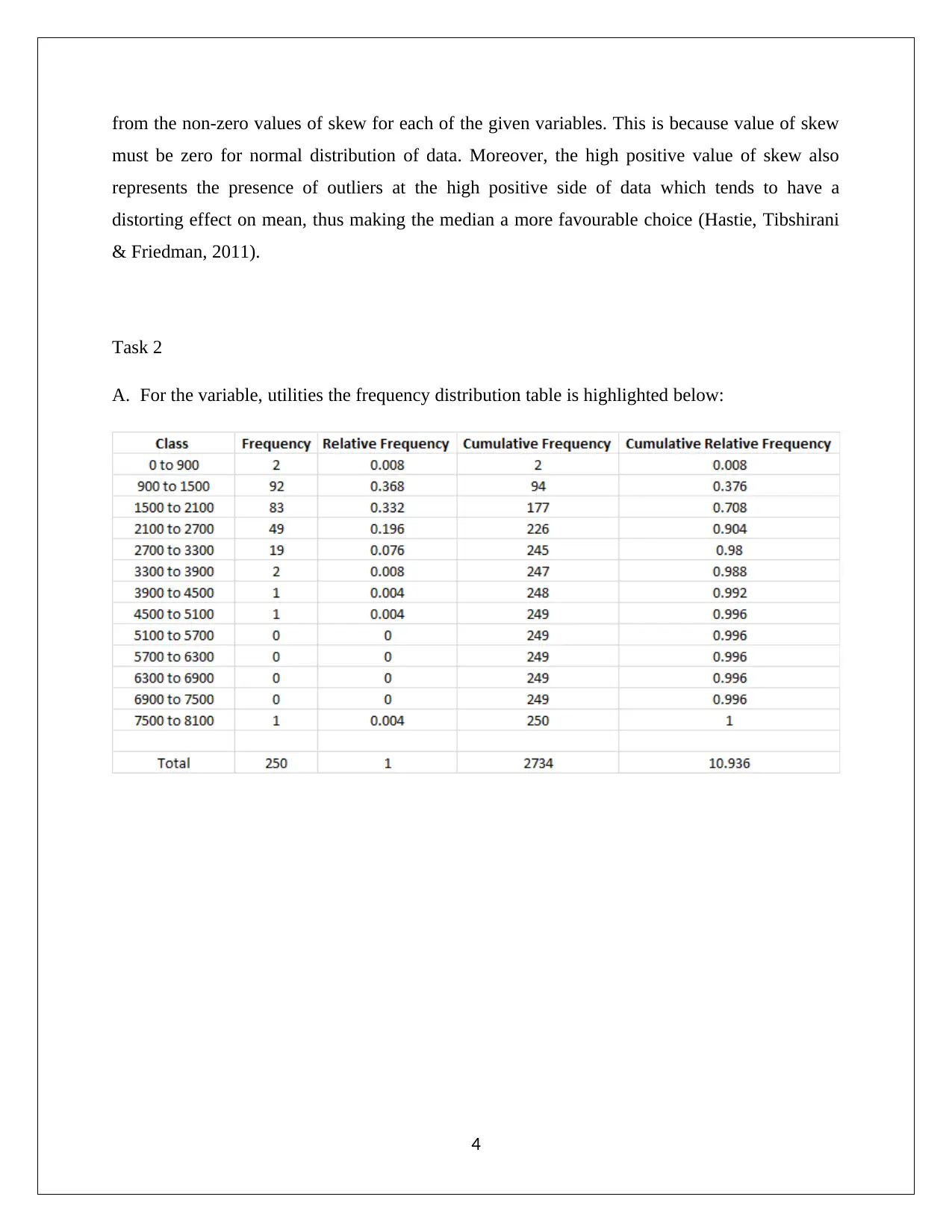
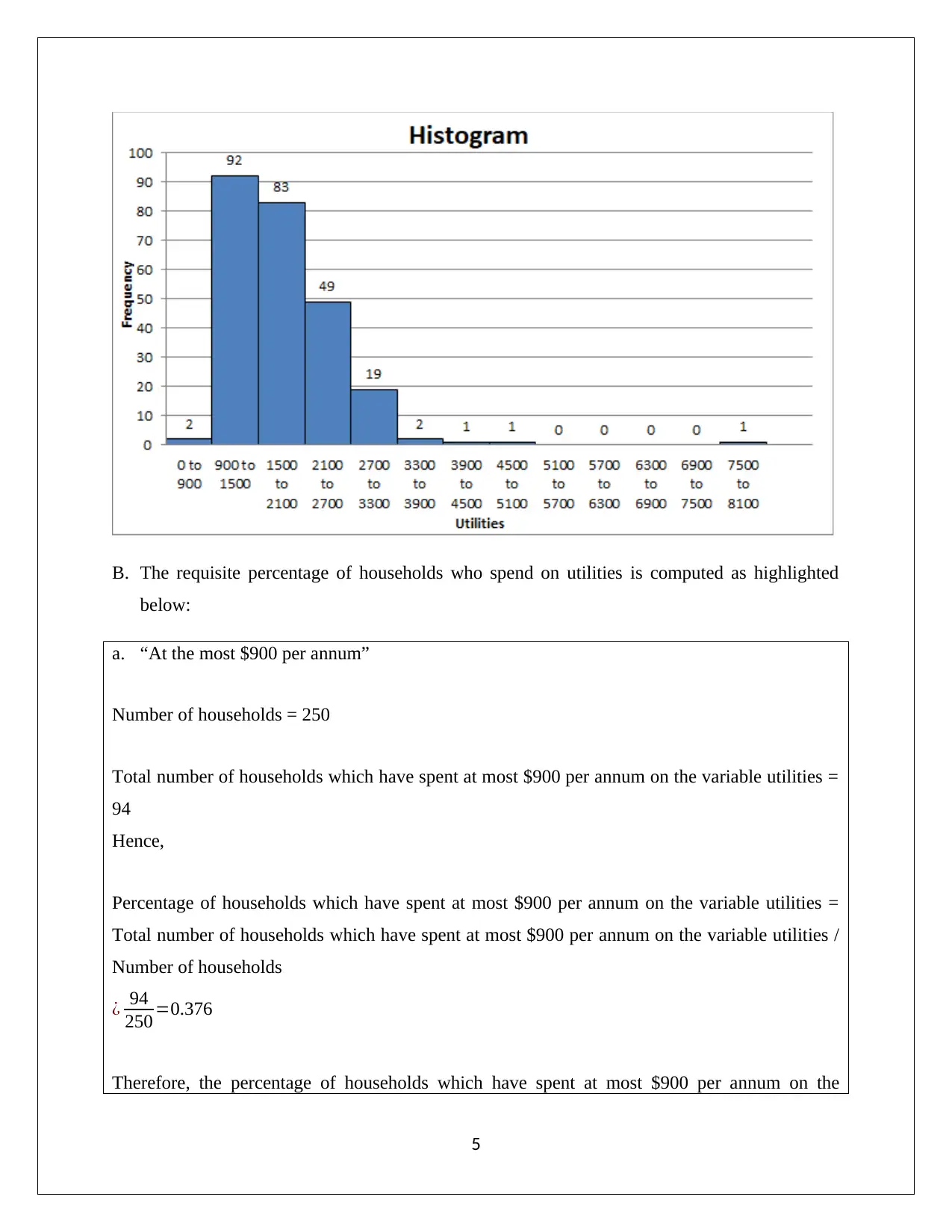
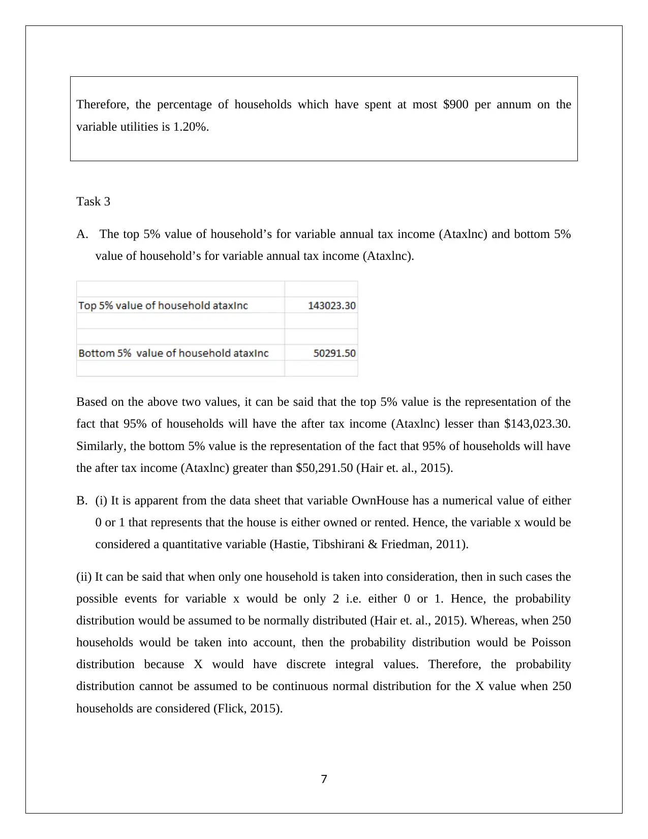
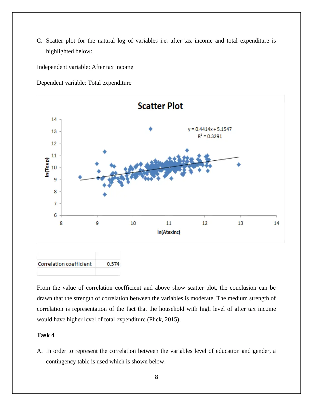
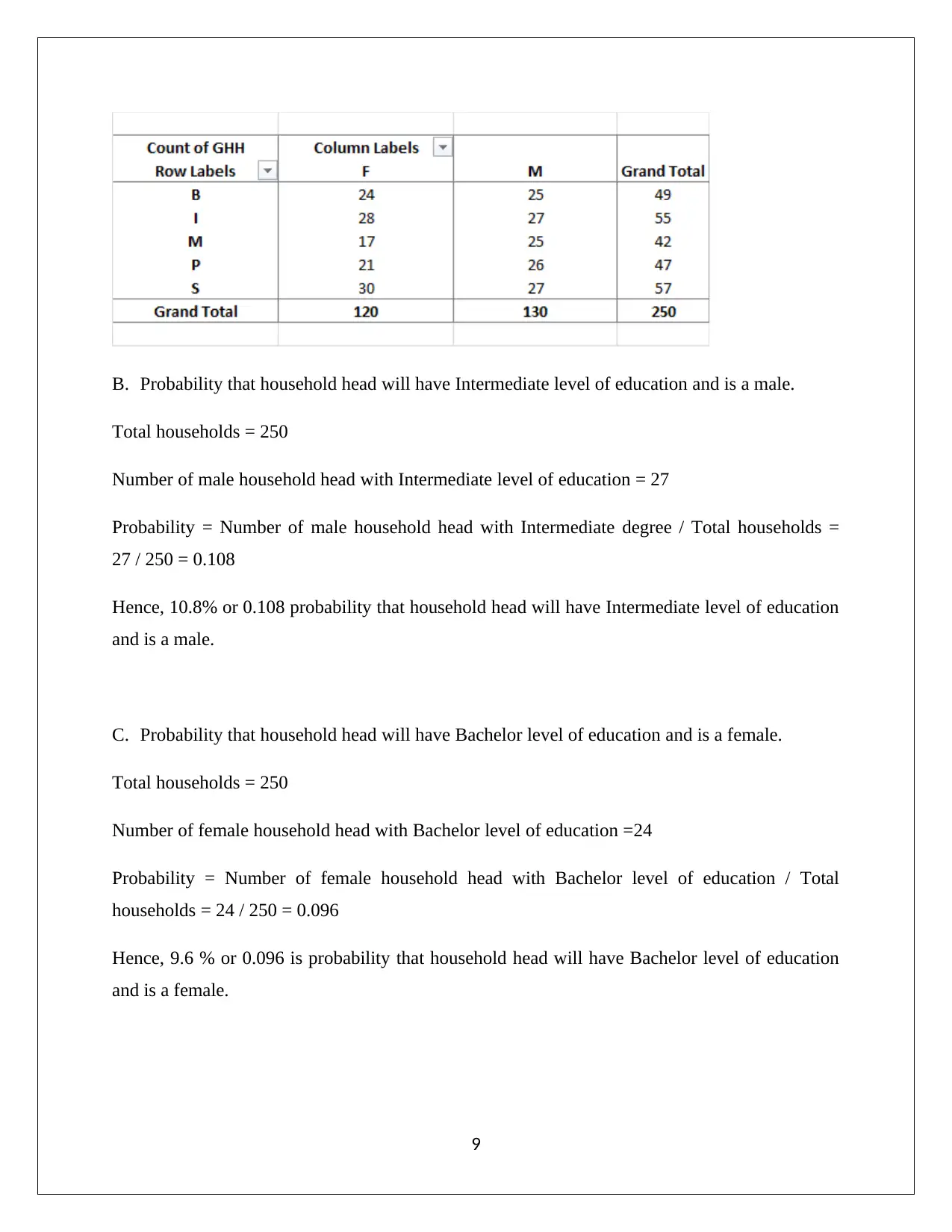
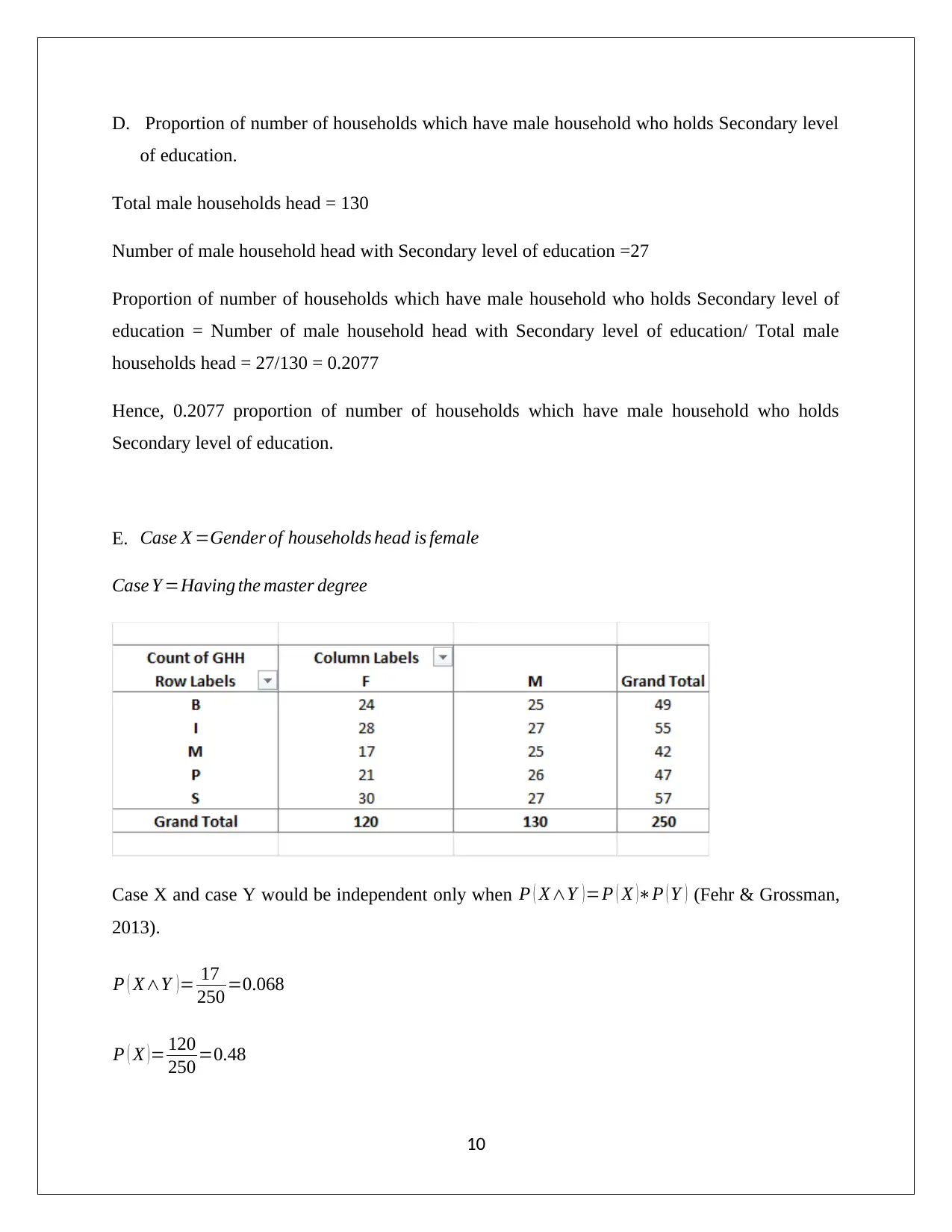
This report presents a comprehensive statistical analysis of household data, addressing various aspects such as sampling methods, descriptive statistics, frequency distributions, and correlation analysis. It begins by evaluating the appropriateness of simple random sampling and suggests stratified random sampling for better representation. Descriptive statistics and box-whisker plots are used to analyze variables like alcohol, meals, fuel, and phone expenses, revealing non-normal data distributions and the presence of outliers. The report then examines household spending on utilities, calculating percentages for different expenditure ranges. Further analysis includes determining top and bottom 5% values for after-tax income and discussing the probability distributions of household characteristics. Correlation between after-tax income and total expenditure is assessed using scatter plots and correlation coefficients. Finally, the report explores the relationship between education level and gender using contingency tables and probability calculations, concluding with an assessment of independence between variables. This assignment solution is available on Desklib, a platform offering a wealth of study resources for students.

BUS5SBF Statistics For Business and Finance
Analyzing Household Data
Student Name
[Pick the date]

Task 1
A. The requisite sampling method that has been used is simple random sampling. In this
sampling method, there is an equal probability associated with the selection of each element.
A key concern in this sampling method is the under-representation and over-representation of
key population attributes especially taking into cognizance the low sample size (Eriksson &
Kovalainen, 2015). Thus, it would be better to sue stratified random sampling since it would
ensure that there is fair representation of the important population attributes. This method
involves classification of population as per key attributes as the first step which is followed by
random sampling of requisite individuals from each group who are selected in the same ratio
as they are present in the population.(Flick, 2015).
B. Descriptive statistics along with the Box- whisker plot for the variables (Alcohol, meals, fuel
and phone) is given below:
Descriptive statistics
1

2

Box- whisker plot
C. Based on the descriptive statistics, it can be seen that for all the four variables the measures of
central tendency i.e. mean median and modes are not same. This indicates that the distribution of
data is not normal and thus shape can be assumed to be asymmetric. Further, this is also evident
3

from the non-zero values of skew for each of the given variables. This is because value of skew
must be zero for normal distribution of data. Moreover, the high positive value of skew also
represents the presence of outliers at the high positive side of data which tends to have a
distorting effect on mean, thus making the median a more favourable choice (Hastie, Tibshirani
& Friedman, 2011).
Task 2
A. For the variable, utilities the frequency distribution table is highlighted below:
4

B. The requisite percentage of households who spend on utilities is computed as highlighted
below:
a. “At the most $900 per annum”
Number of households = 250
Total number of households which have spent at most $900 per annum on the variable utilities =
94
Hence,
Percentage of households which have spent at most $900 per annum on the variable utilities =
Total number of households which have spent at most $900 per annum on the variable utilities /
Number of households
¿ 94
250 =0.376
Therefore, the percentage of households which have spent at most $900 per annum on the
5

variable utilities is 37.6%.
b. “Between $1500 and $2700 per annum”
Number of households = 250
Total number of households which have spent between $1500 and $2700 per annum on the
variable utilities = 83+49 = 132
Hence,
Percentage of households which have spent between $1500 and $2700 per annum on the
variable utilities = Total number of households which have spent between $1500 and $2700 per
annum on the variable utilities / Number of households
¿ 132
250 =0.528
Therefore, the percentage of households has spent between $1500 and $2700 per annum on the
variable utilities 52.80%.
c. “More than $3000 per annum”
Number of households = 250
Total number of households which have spent more than $3000 per annum on the variable
utilities = 3
Hence,
Percentage of households which have spent more than $3000 per annum on the variable utilities
= Total number of households which have spent more than $3000 per annum on the variable
utilities / Number of households
¿ 3
250 =0.012
6

Therefore, the percentage of households which have spent at most $900 per annum on the
variable utilities is 1.20%.
Task 3
A. The top 5% value of household’s for variable annual tax income (Ataxlnc) and bottom 5%
value of household’s for variable annual tax income (Ataxlnc).
Based on the above two values, it can be said that the top 5% value is the representation of the
fact that 95% of households will have the after tax income (Ataxlnc) lesser than $143,023.30.
Similarly, the bottom 5% value is the representation of the fact that 95% of households will have
the after tax income (Ataxlnc) greater than $50,291.50 (Hair et. al., 2015).
B. (i) It is apparent from the data sheet that variable OwnHouse has a numerical value of either
0 or 1 that represents that the house is either owned or rented. Hence, the variable x would be
considered a quantitative variable (Hastie, Tibshirani & Friedman, 2011).
(ii) It can be said that when only one household is taken into consideration, then in such cases the
possible events for variable x would be only 2 i.e. either 0 or 1. Hence, the probability
distribution would be assumed to be normally distributed (Hair et. al., 2015). Whereas, when 250
households would be taken into account, then the probability distribution would be Poisson
distribution because X would have discrete integral values. Therefore, the probability
distribution cannot be assumed to be continuous normal distribution for the X value when 250
households are considered (Flick, 2015).
7

C. Scatter plot for the natural log of variables i.e. after tax income and total expenditure is
highlighted below:
Independent variable: After tax income
Dependent variable: Total expenditure
From the value of correlation coefficient and above show scatter plot, the conclusion can be
drawn that the strength of correlation between the variables is moderate. The medium strength of
correlation is representation of the fact that the household with high level of after tax income
would have higher level of total expenditure (Flick, 2015).
Task 4
A. In order to represent the correlation between the variables level of education and gender, a
contingency table is used which is shown below:
8

B. Probability that household head will have Intermediate level of education and is a male.
Total households = 250
Number of male household head with Intermediate level of education = 27
Probability = Number of male household head with Intermediate degree / Total households =
27 / 250 = 0.108
Hence, 10.8% or 0.108 probability that household head will have Intermediate level of education
and is a male.
C. Probability that household head will have Bachelor level of education and is a female.
Total households = 250
Number of female household head with Bachelor level of education =24
Probability = Number of female household head with Bachelor level of education / Total
households = 24 / 250 = 0.096
Hence, 9.6 % or 0.096 is probability that household head will have Bachelor level of education
and is a female.
9

D. Proportion of number of households which have male household who holds Secondary level
of education.
Total male households head = 130
Number of male household head with Secondary level of education =27
Proportion of number of households which have male household who holds Secondary level of
education = Number of male household head with Secondary level of education/ Total male
households head = 27/130 = 0.2077
Hence, 0.2077 proportion of number of households which have male household who holds
Secondary level of education.
E. Case X =Gender of households head is female
Case Y =Having the master degree
Case X and case Y would be independent only when P ( X∧Y )=P ( X )∗P ( Y ) (Fehr & Grossman,
2013).
P ( X∧Y )= 17
250 =0.068
P ( X )= 120
250 =0.48
10

P ( Y )= 42
250 =0.168
Hence,
P ( X∧Y )=P ( X )∗P ( Y )
0.068=0.48∗0.168
0.068 ≠ 0.08064
P ( X∧Y ) ≠ P ( X )∗P ( Y )
It is apparent that the above condition is not satisfied and thus, the cases (having master degree
and female household head) are not independent.
References
Eriksson, P. & Kovalainen, A. (2015) Quantitative methods in business research (3rd ed.).
London: Sage Publications.
Fehr, F. H., & Grossman, G. (2013) An introduction to sets, probability and hypothesis testing
(3rd ed.). Ohio: Heath.
Flick, U. (2015) Introducing research methodology: A beginner's guide to doing a research
project (4th ed.). New York: Sage Publications.
Hair, J. F., Wolfinbarger, M., Money, A. H., Samouel, P., & Page, M. J. (2015) Essentials of
business research methods (2nd ed.). New York: Routledge.
Hastie, T., Tibshirani, R. & Friedman, J. (2011) The Elements of Statistical Learning (4th
ed.). New York: Springer Publications.
11