BUS5SBF - Statistics for Finance: Household Data Analysis Report

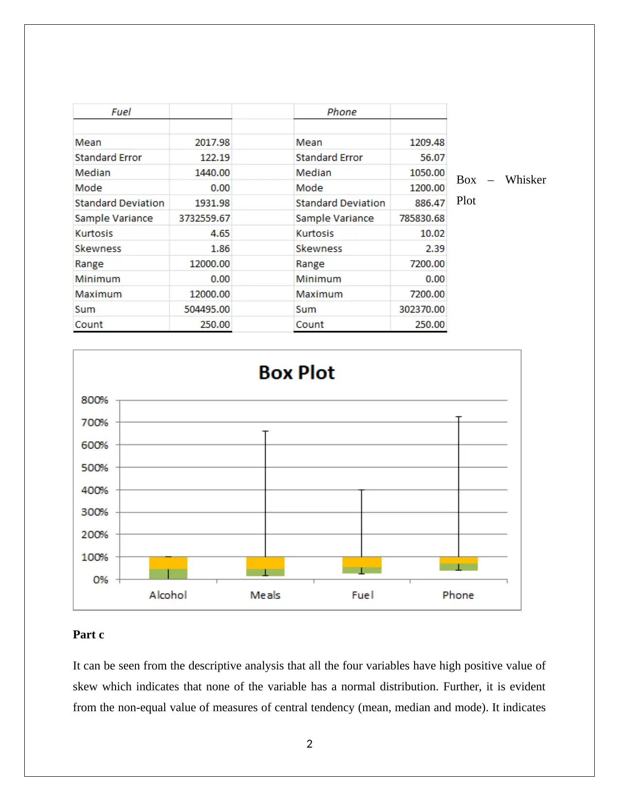
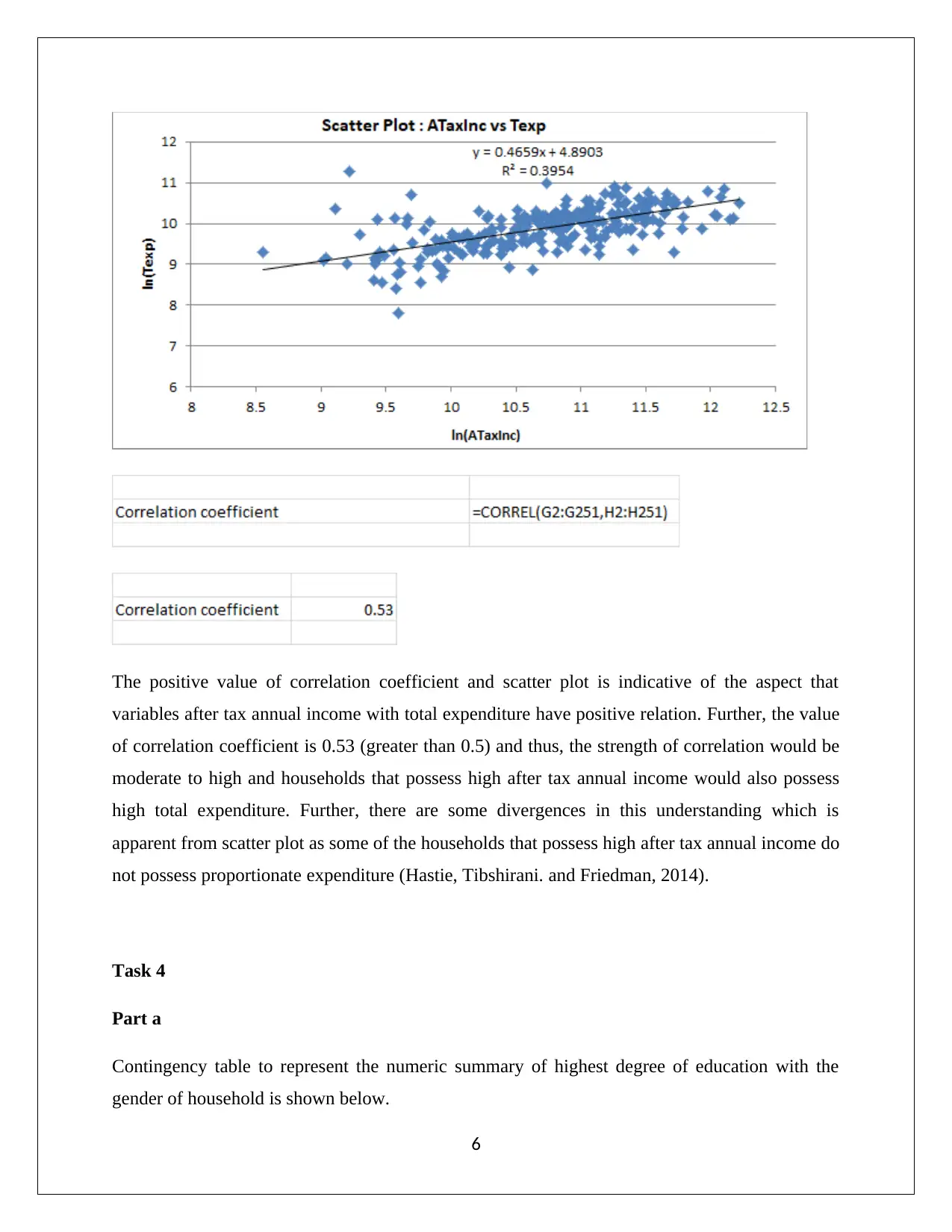
This report presents a statistical analysis of household data, employing simple random sampling and stratified random sampling techniques. It includes numerical summaries of variables like alcohol, meal, fuel, and phone expenses, revealing skewed distributions and suggesting the use of median as a central tendency measure. The analysis further examines household spending on utilities, calculates top and bottom income percentages, and classifies household ownership variables. Correlation analysis between after-tax income and total expenditure is performed, indicating a moderate to high positive relationship. Finally, the report includes a contingency table summarizing education levels and gender, calculating probabilities, and determining the independence of gender and education events. The report uses statistical methods to interpret demographic data, demonstrating the real-world applications of statistics in finance and business contexts. This document is available on Desklib, a platform offering a wide range of study resources for students.

Statistics For Business and Finance
[Pick the date]
Student Name

TASK 1
Part a
In the present scenario, simple random sampling technique has been taken into consideration to
take the sample from the given population. The probability of selecting each element is same in
case of simple random sampling. In this sampling, the sample would not show the true
representation of population and deviate from the actual distribution of the population. This
would happen since the underlying attributes such as gender, education would not have the same
representation in the sample as the population (Hair et. al., 2015). Therefore, it would be
appropriate to use stratified random sampling technique in regards to take a sample of 250 from
the population. The derived sample would be true representative of population because the
sample would be derived randomly after the population has been divided based on their central
attributes. In such case, the sample would comprise the attributes in the same proportion as the
population (Eriksson and Kovalainen, 2015).
Part b
Numerical summary of variables (Alcohol, meal, fuel and phone) is shown below.
1

Box – Whisker
Plot
Part c
It can be seen from the descriptive analysis that all the four variables have high positive value of
skew which indicates that none of the variable has a normal distribution. Further, it is evident
from the non-equal value of measures of central tendency (mean, median and mode). It indicates
2

that some of the individuals have spent abnormally high amount on alcohol, meals, fuel and
phone. Also, the appropriate measure of central tendency would be median rather than mean
because mean can be distorted as evident from box plot. Further, in regards to measure the
variability of the variables, coefficient of variation should be taken into consideration (Flick,
2015).
Task 2
Part a
Frequency table for utilities
Part b
(a) % of household that spent at most $900 annually on utilities
Households that spent at most $900 annually on utilities = 27 +36 +42 = 105
Total households =250
% of household that spent at most $900 annually on utilities = Households that spent at most
$900 annually on utilities/ Total households = 105 /250 = 0.42 or 42%
3

(b) % of household that spent between $1500 and $2700 annually on utilities
Households that spent between $1500 and $2700 annually on utilities = 27 +14+10+4 = 55
Total households =250
% of household that spent between $1500 and $2700 annually on utilities = Households that
spent between $1500 and $2700 annually on utilities / Total households = 55 /250 = 0.22 or 22%
(c) % of household that spent more than $3000 annually on utilities
Households that spent more than $3000 annually on utilities = 6
Total households =250
% of household that spent more than $3000 annually on utilities = Households that spent more
than $3000 annually on utilities / Total households = 6 /250 = 0.024 or 2.4%
TASK 3
Part a
Top 5% and bottom 5% value of annual after tax income of the households are calculated as
shown below.
4

Top 5% value: It indicates that 95% of the total households would hold an annual after tax
income lesser than or same as $124224.75.
Bottom 5 % value: It indicates that 95% of the total households would hold an annual after tax
income greater than or same as $49894.5.
Part b
(i) X indicates the total household who has owned a house or rented the house. It can be said
that there are only two expected outcomes of variable X which are as follows.
X =1 ( Owned the house )
X =0( Rented the house)
The variable would be classified as qualitative variable irrespective of the numerical magnitude
because the numeric number is the representation of a holding the house or renting the house
(Hillier, 2016).
(ii) Case when single household needs to be analysed, then the possible outcomes will be
either 1 or 0. Hence, probability distribution would be classified as binomial distribution.
On the other hand, when 250 households need to be analysed, then there would be set of
discrete integral results (positive) and hence, the distribution would be known as Poisson
distribution (Hair et. al., 2015).
Part c
Scatter plot and correlation coefficient to represent the association between after tax annual
income with total expenditure is highlighted below.
5

The positive value of correlation coefficient and scatter plot is indicative of the aspect that
variables after tax annual income with total expenditure have positive relation. Further, the value
of correlation coefficient is 0.53 (greater than 0.5) and thus, the strength of correlation would be
moderate to high and households that possess high after tax annual income would also possess
high total expenditure. Further, there are some divergences in this understanding which is
apparent from scatter plot as some of the households that possess high after tax annual income do
not possess proportionate expenditure (Hastie, Tibshirani. and Friedman, 2014).
Task 4
Part a
Contingency table to represent the numeric summary of highest degree of education with the
gender of household is shown below.
6

Part b
Probability that head of household would be male and hold Intermediate degree =?
Total households =250
Household would be male and hold Intermediate degree = 25
Probability that head of household would be male and hold Intermediate degree =25 /250 = 0.1
Part c
Probability that head of household would be female and hold Bachelor degree =?
Total households =250
Household would be female and hold Bachelor degree = 23
Probability that head of household would be female and hold Bachelor degree =23 /250 = 0.092
Part d
The proportion of household with male head and hold Secondary degree =?
Total households =250
Household with male head and hold Secondary degree =32
7

The proportion of household with male head and hold Secondary degree =32/250 = 0.128
Part e
Events (A, B) are said to be independent when P (A and B) =P (A). P (B)
Let Event A is female household head, P (A) = 126/250= 0.504
Event B is Master degree as highest degree of education, P (B) =46/250 =0.184
Now,
P (A). P (B) =0.504*0.184 = 0.0927
Household with female head and master degree, P (A and B) = 33/250 = 0.132
It is clear that P( A∧B)≠ P (A ). P( B)
0.0927 ≠ 0.132
Therefore, ‘gender and education degree are not independent events.’
8

References
Eriksson, P. and Kovalainen, A. (2015) Quantitative methods in business research. 3rd ed.
London: Sage Publications.
Flick, U. (2015) Introducing research methodology: A beginner's guide to doing a research
project. 4th ed. New York: Sage Publications.
Hair, J. F., Wolfinbarger, M., Money, A. H., Samouel, P., and Page, M. J. (2015) Essentials of
business research methods. 2nd ed. New York: Routledge.
Hastie, T., Tibshirani, R. and Friedman, J. (2014) The Elements of Statistical Learning. 4th
ed. New York: Springer Publications.
Hillier, F. (2016) Introduction to Operations Research. 6th ed. New York: McGraw Hill
Publications.
9