BUS708 Statistics and Data Analysis: Airline Services Report
VerifiedAdded on 2023/04/21
|9
|2400
|97
Report
AI Summary
This report analyzes airline services in Australia using statistical methods. It examines international flight data, focusing on flight frequencies and airport usage. The analysis includes hypothesis testing to determine if the average monthly flights exceed 30 and if there is a significant association between selected Australian airports and airlines. The report uses both primary data collected from a survey of KOI students and secondary data from a sample of 1000 international flights. The findings indicate an asymmetric distribution of flight frequencies and no statistically significant association between airports and airlines. Melbourne is identified as the airport with the highest traffic from the selected airlines. The report concludes with recommendations for future research, emphasizing the need to study specific passenger groups to understand their airport preferences.

STATISTICS
STUDENT ID:
[Pick the date]
STUDENT ID:
[Pick the date]
Paraphrase This Document
Need a fresh take? Get an instant paraphrase of this document with our AI Paraphraser
Section 1: Introduction
a) The significance of this report needs to analysed in the given context where in Australia, there is
increased international traffic. Further, another interesting development is that there is a rising
market share of international airlines with regards to international travel originating or ending in
Australia. The market share growth rate comparison for domestic and international players tends to
provide testimony to the above statement. A contributing factor to the higher growth rate of
international carriers may be attributed to capacity cutting by Qantas as an efficiency measure for
improving occupancy (AnnaAero, 2018). For capturing this increasing market, it is imperative that
the Australian airports need to understand the preferences and needs of the consumers and make
suitable adjustments.
b) Dataset 1 highlights the information of the sample of 1000 international flights that have any
Australian city as the source or the destination. This dataset has several variables pertaining to these
flights related to information regarding source, destination, route, frequency of given flight in a
month, stops count and maximum seats available. This data of 1000 flights would be considered as
secondary data as this data is not collected myself but has been obtained from an external source by
the University. While the dataset has a host of variables, a significant amount of these are non-
numerical variables which are labelled as categorical variables. These are represented in the dataset
with the use of nominal measurement scale. But some variables are there in the dataset which have
numerical values and are thus not categorical which have used ratio scale for measurement (Hastie,
Tibshirani and Friedman, 2014). The typical cases for the dataset would be driven by the underlying
population which essentially constitutes of every international flight during the given period flying
from or to Australia.
c) Dataset 2 comprises of primary data which is different from dataset 1. This data is termed as
primary as the underlying data represented has been collected through conducted survey by myself
and the underlying data has not been copied from any other source. The respondents (35 in total)
for the requisite survey were KOI students. Unlike dataset 1, this dataset 2 offers scope that is les
wider as instead of multiple variables expressed in dataset 1, just three variables are included here
i.e. city in Australia, Airline and city abroad. For the given variables, the underlying data
measurement technique is nominal considering categorical data that cannot be automatically
arranged in any order. The reliability of the conclusions based on the given data may be adversely
impacted on account of use of non-probability sampling technique where instead of choosing KOI
students randomly these were chosen driven by own convenience. This may have led to the sample
being bias thereby impacting the overall reliability (Fehr and Grossman, 2013).
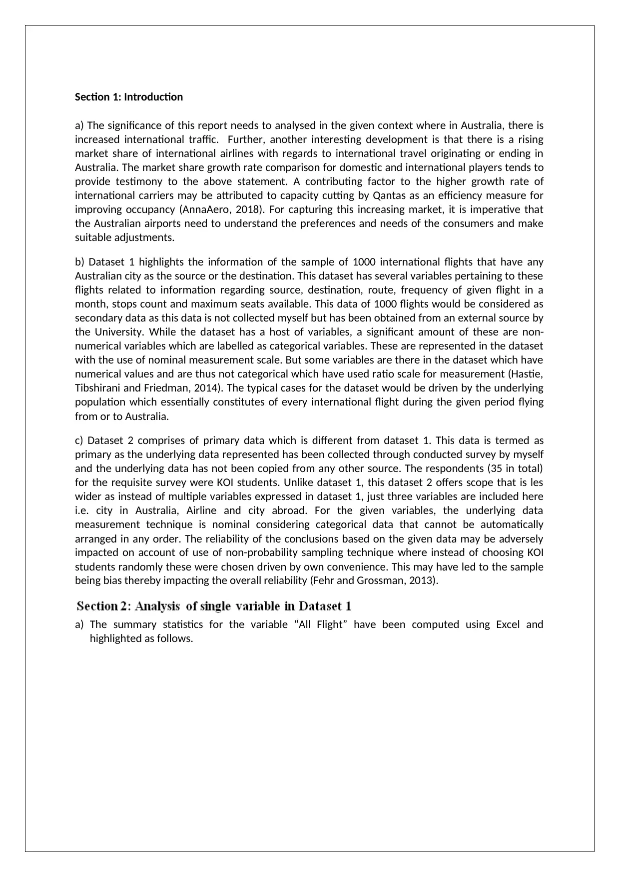
a) The summary statistics for the variable “All Flight” have been computed using Excel and
highlighted as follows.
a) The significance of this report needs to analysed in the given context where in Australia, there is
increased international traffic. Further, another interesting development is that there is a rising
market share of international airlines with regards to international travel originating or ending in
Australia. The market share growth rate comparison for domestic and international players tends to
provide testimony to the above statement. A contributing factor to the higher growth rate of
international carriers may be attributed to capacity cutting by Qantas as an efficiency measure for
improving occupancy (AnnaAero, 2018). For capturing this increasing market, it is imperative that
the Australian airports need to understand the preferences and needs of the consumers and make
suitable adjustments.
b) Dataset 1 highlights the information of the sample of 1000 international flights that have any
Australian city as the source or the destination. This dataset has several variables pertaining to these
flights related to information regarding source, destination, route, frequency of given flight in a
month, stops count and maximum seats available. This data of 1000 flights would be considered as
secondary data as this data is not collected myself but has been obtained from an external source by
the University. While the dataset has a host of variables, a significant amount of these are non-
numerical variables which are labelled as categorical variables. These are represented in the dataset
with the use of nominal measurement scale. But some variables are there in the dataset which have
numerical values and are thus not categorical which have used ratio scale for measurement (Hastie,
Tibshirani and Friedman, 2014). The typical cases for the dataset would be driven by the underlying
population which essentially constitutes of every international flight during the given period flying
from or to Australia.
c) Dataset 2 comprises of primary data which is different from dataset 1. This data is termed as
primary as the underlying data represented has been collected through conducted survey by myself
and the underlying data has not been copied from any other source. The respondents (35 in total)
for the requisite survey were KOI students. Unlike dataset 1, this dataset 2 offers scope that is les
wider as instead of multiple variables expressed in dataset 1, just three variables are included here
i.e. city in Australia, Airline and city abroad. For the given variables, the underlying data
measurement technique is nominal considering categorical data that cannot be automatically
arranged in any order. The reliability of the conclusions based on the given data may be adversely
impacted on account of use of non-probability sampling technique where instead of choosing KOI
students randomly these were chosen driven by own convenience. This may have led to the sample
being bias thereby impacting the overall reliability (Fehr and Grossman, 2013).
a) The summary statistics for the variable “All Flight” have been computed using Excel and
highlighted as follows.
With regards to shape, one of the most crucial parameters is the skew which is positive and quite
high in value. This implies that while majority of data points would be represented at the lower end
but there would exist some data points which are eexceptionally large and would lead to a lengthy
tail on the right of the mean. This conclusion is supported from the fact that the mean is 24.56, the
maximum value is 162 which clearly imply that outliers may be present in the data on the higher
side. However, this high range is on expected lines owing to traffic demand varying significantly on
different sectors because of which the number of flights operating on the sector would also vary.
Hence, the underlying shape of the distribution of “All Flight” would be asymmetric owing to
presence of a large skew.
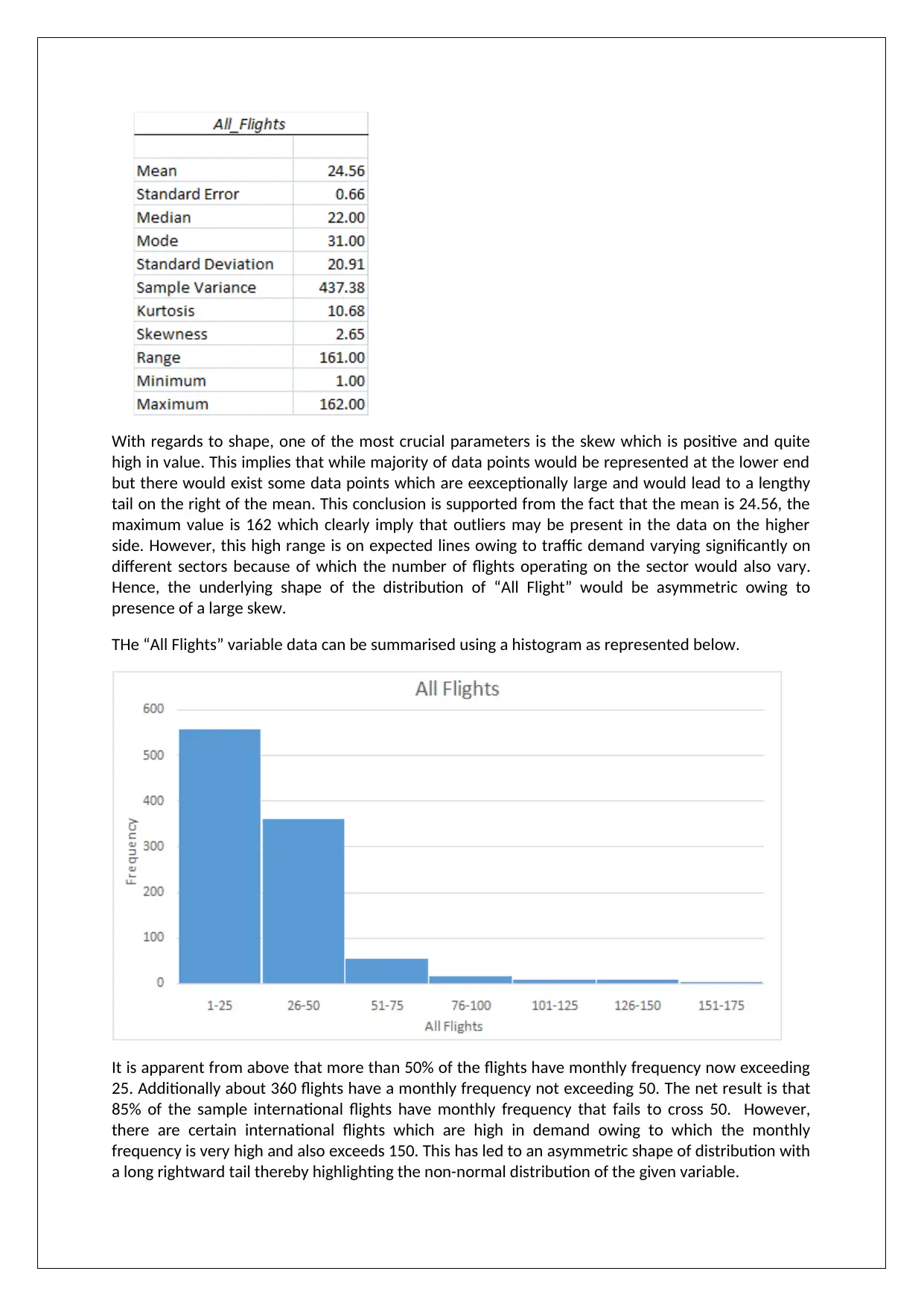
THe “All Flights” variable data can be summarised using a histogram as represented below.
It is apparent from above that more than 50% of the flights have monthly frequency now exceeding
25. Additionally about 360 flights have a monthly frequency not exceeding 50. The net result is that
85% of the sample international flights have monthly frequency that fails to cross 50. However,
there are certain international flights which are high in demand owing to which the monthly
frequency is very high and also exceeds 150. This has led to an asymmetric shape of distribution with
a long rightward tail thereby highlighting the non-normal distribution of the given variable.
high in value. This implies that while majority of data points would be represented at the lower end
but there would exist some data points which are eexceptionally large and would lead to a lengthy
tail on the right of the mean. This conclusion is supported from the fact that the mean is 24.56, the
maximum value is 162 which clearly imply that outliers may be present in the data on the higher
side. However, this high range is on expected lines owing to traffic demand varying significantly on
different sectors because of which the number of flights operating on the sector would also vary.
Hence, the underlying shape of the distribution of “All Flight” would be asymmetric owing to
presence of a large skew.
THe “All Flights” variable data can be summarised using a histogram as represented below.
It is apparent from above that more than 50% of the flights have monthly frequency now exceeding
25. Additionally about 360 flights have a monthly frequency not exceeding 50. The net result is that
85% of the sample international flights have monthly frequency that fails to cross 50. However,
there are certain international flights which are high in demand owing to which the monthly
frequency is very high and also exceeds 150. This has led to an asymmetric shape of distribution with
a long rightward tail thereby highlighting the non-normal distribution of the given variable.
⊘ This is a preview!⊘
Do you want full access?
Subscribe today to unlock all pages.
Trusted by 1+ million students worldwide
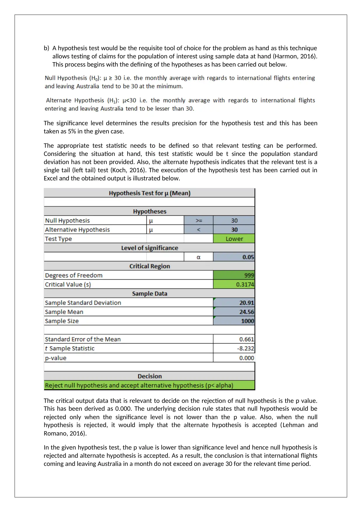
b) A hypothesis test would be the requisite tool of choice for the problem as hand as this technique
allows testing of claims for the population of interest using sample data at hand (Harmon, 2016).
This process begins with the defining of the hypotheses as has been carried out below.
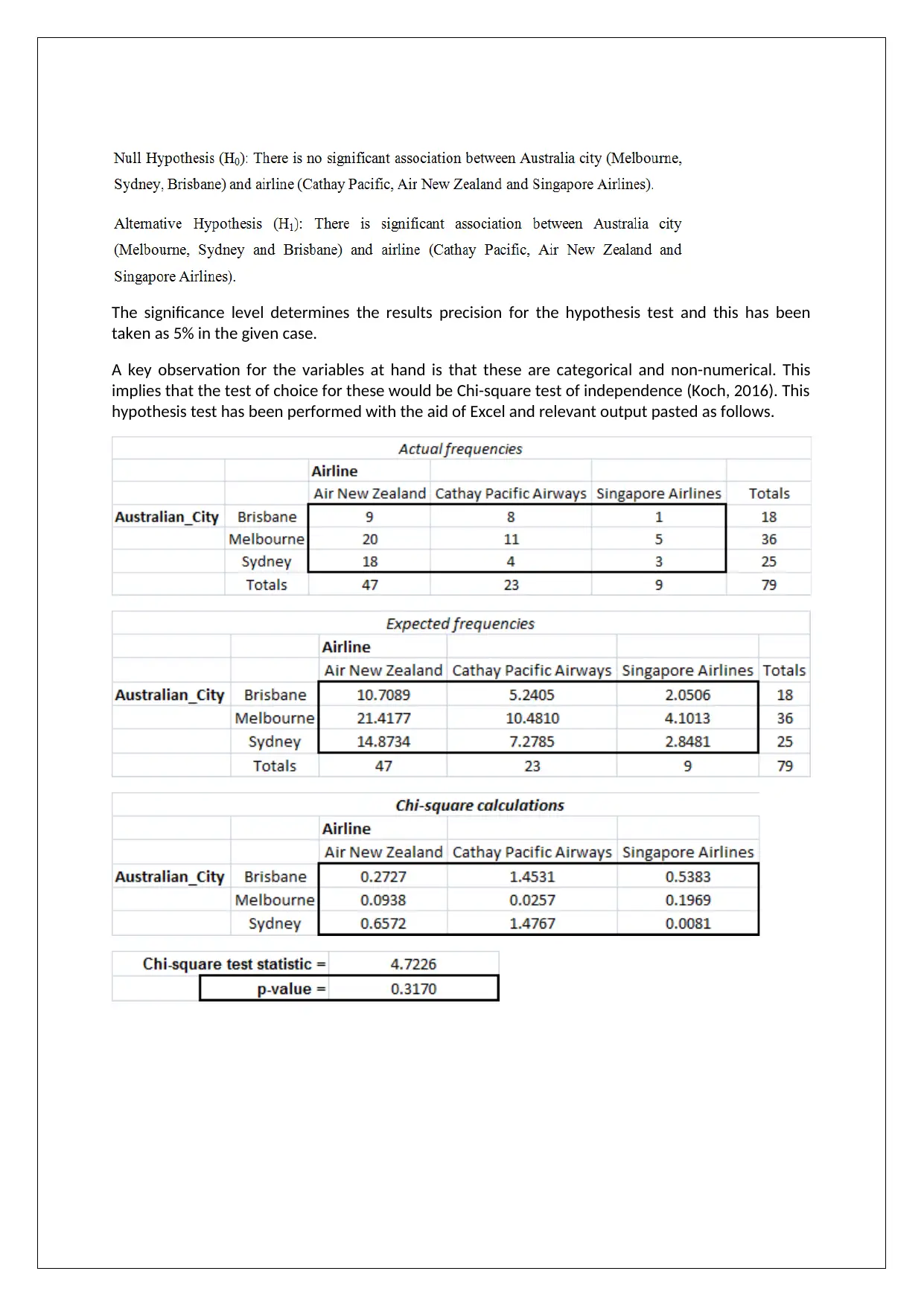
The significance level determines the results precision for the hypothesis test and this has been
taken as 5% in the given case.
The appropriate test statistic needs to be defined so that relevant testing can be performed.
Considering the situation at hand, this test statistic would be t since the population standard
deviation has not been provided. Also, the alternate hypothesis indicates that the relevant test is a
single tail (left tail) test (Koch, 2016). The execution of the hypothesis test has been carried out in
Excel and the obtained output is illustrated below.
The critical output data that is relevant to decide on the rejection of null hypothesis is the p value.
This has been derived as 0.000. The underlying decision rule states that null hypothesis would be
rejected only when the significance level is not lower than the p value. Also, when the null
hypothesis is rejected, it would imply that the alternate hypothesis is accepted (Lehman and
Romano, 2016).
In the given hypothesis test, the p value is lower than significance level and hence null hypothesis is
rejected and alternate hypothesis is accepted. As a result, the conclusion is that international flights
coming and leaving Australia in a month do not exceed on average 30 for the relevant time period.
allows testing of claims for the population of interest using sample data at hand (Harmon, 2016).
This process begins with the defining of the hypotheses as has been carried out below.
The significance level determines the results precision for the hypothesis test and this has been
taken as 5% in the given case.
The appropriate test statistic needs to be defined so that relevant testing can be performed.
Considering the situation at hand, this test statistic would be t since the population standard
deviation has not been provided. Also, the alternate hypothesis indicates that the relevant test is a
single tail (left tail) test (Koch, 2016). The execution of the hypothesis test has been carried out in
Excel and the obtained output is illustrated below.
The critical output data that is relevant to decide on the rejection of null hypothesis is the p value.
This has been derived as 0.000. The underlying decision rule states that null hypothesis would be
rejected only when the significance level is not lower than the p value. Also, when the null
hypothesis is rejected, it would imply that the alternate hypothesis is accepted (Lehman and
Romano, 2016).
In the given hypothesis test, the p value is lower than significance level and hence null hypothesis is
rejected and alternate hypothesis is accepted. As a result, the conclusion is that international flights
coming and leaving Australia in a month do not exceed on average 30 for the relevant time period.
Paraphrase This Document
Need a fresh take? Get an instant paraphrase of this document with our AI Paraphraser
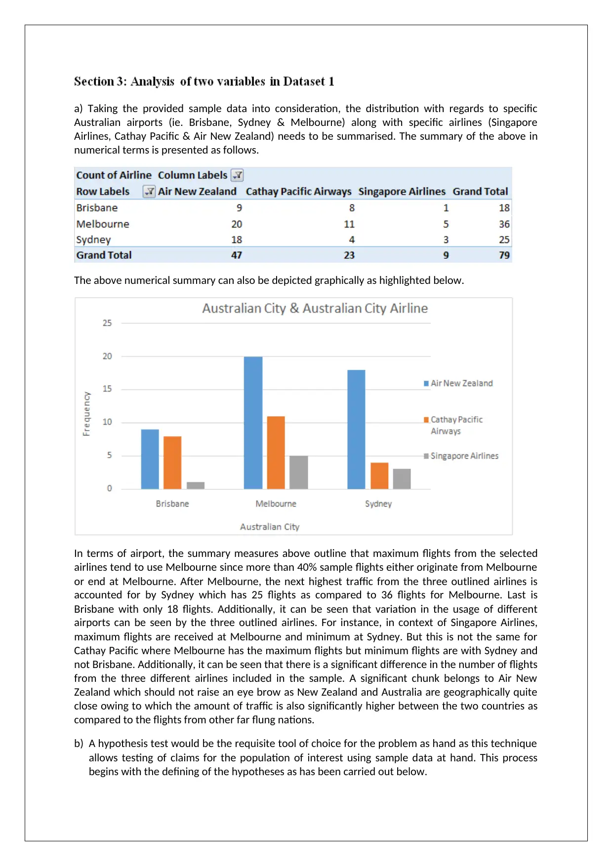
a) Taking the provided sample data into consideration, the distribution with regards to specific
Australian airports (ie. Brisbane, Sydney & Melbourne) along with specific airlines (Singapore
Airlines, Cathay Pacific & Air New Zealand) needs to be summarised. The summary of the above in
numerical terms is presented as follows.
The above numerical summary can also be depicted graphically as highlighted below.
In terms of airport, the summary measures above outline that maximum flights from the selected
airlines tend to use Melbourne since more than 40% sample flights either originate from Melbourne
or end at Melbourne. After Melbourne, the next highest traffic from the three outlined airlines is
accounted for by Sydney which has 25 flights as compared to 36 flights for Melbourne. Last is
Brisbane with only 18 flights. Additionally, it can be seen that variation in the usage of different
airports can be seen by the three outlined airlines. For instance, in context of Singapore Airlines,
maximum flights are received at Melbourne and minimum at Sydney. But this is not the same for
Cathay Pacific where Melbourne has the maximum flights but minimum flights are with Sydney and
not Brisbane. Additionally, it can be seen that there is a significant difference in the number of flights
from the three different airlines included in the sample. A significant chunk belongs to Air New
Zealand which should not raise an eye brow as New Zealand and Australia are geographically quite
close owing to which the amount of traffic is also significantly higher between the two countries as
compared to the flights from other far flung nations.
b) A hypothesis test would be the requisite tool of choice for the problem as hand as this technique
allows testing of claims for the population of interest using sample data at hand. This process
begins with the defining of the hypotheses as has been carried out below.
The significance level determines the results precision for the hypothesis test and this has been
taken as 5% in the given case.
A key observation for the variables at hand is that these are categorical and non-numerical. This
implies that the test of choice for these would be Chi-square test of independence (Koch, 2016). This
hypothesis test has been performed with the aid of Excel and relevant output pasted as follows.
⊘ This is a preview!⊘
Do you want full access?
Subscribe today to unlock all pages.
Trusted by 1+ million students worldwide
The critical output data that is relevant to decide on the rejection of null hypothesis is the p value.
This has been derived as 0.000. The underlying decision rule states that null hypothesis would be
rejected only when the significance level is not lower than the p value. Also, when the null
hypothesis is rejected, it would imply that the alternate hypothesis is accepted (Harmon, 2013).
The computed p value from the output above is 0.3170 which exceeds the significance level for the
hypothesis test. This would imply availability of insufficient evidence to warrant null hypothesis
rejection. Hence, alternate hypothesis cannot be accepted. Therefore, it is appropriate to conclude
that level of association between selected Australian airports and the selected airlines is not found
to be statistically significant.
c) As the relation between the Australian airports and respective international airlines is not
statistically significant, therefore the comparison of performance of the airports should be carried
based on the sample data and the amount of traffic from these airports. Taking this into
consideration, the best performer would be Melbourne (36), followed by Sydney (25) and Brisbane
occupying the last position with 18 flights only.
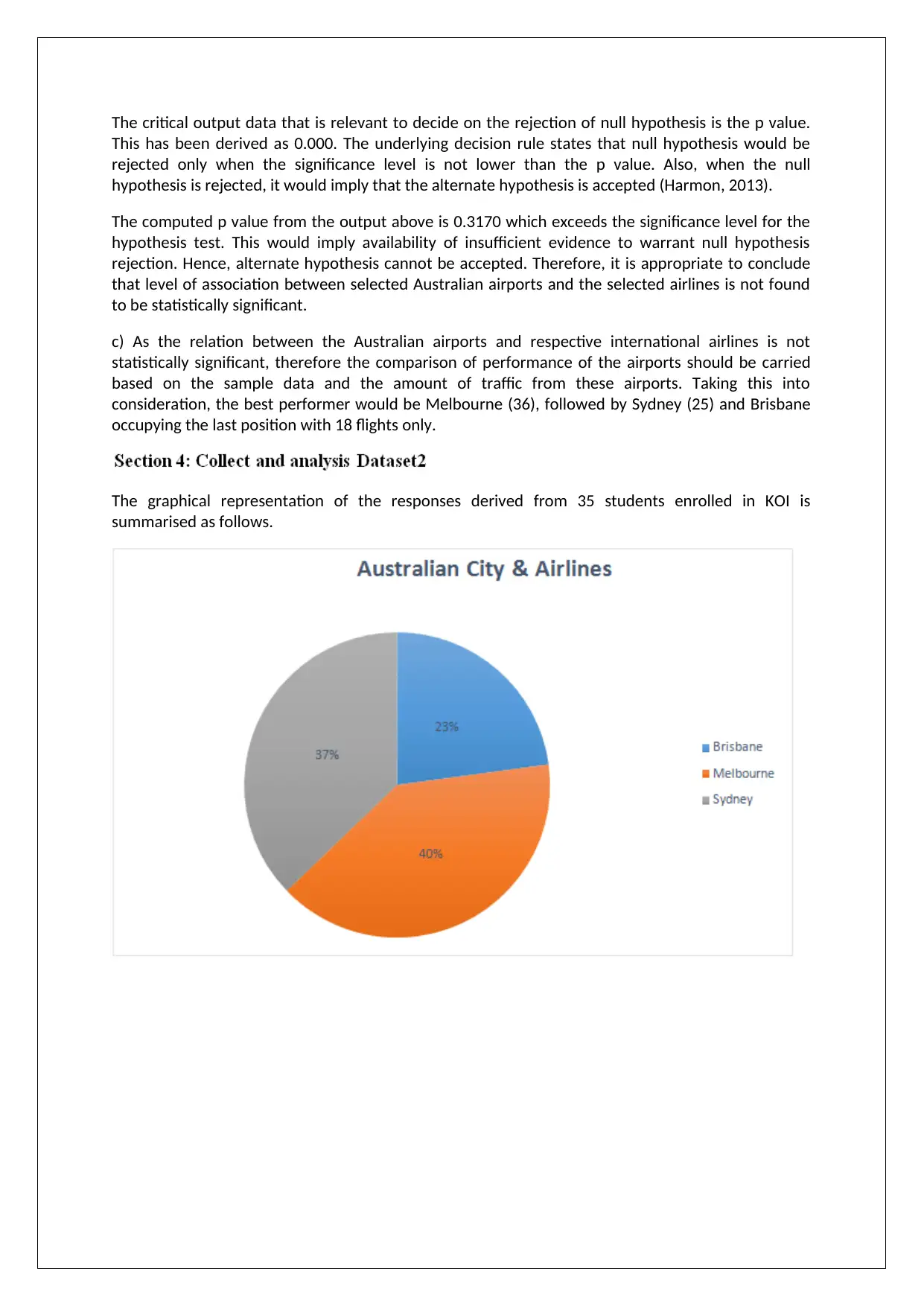
The graphical representation of the responses derived from 35 students enrolled in KOI is
summarised as follows.
This has been derived as 0.000. The underlying decision rule states that null hypothesis would be
rejected only when the significance level is not lower than the p value. Also, when the null
hypothesis is rejected, it would imply that the alternate hypothesis is accepted (Harmon, 2013).
The computed p value from the output above is 0.3170 which exceeds the significance level for the
hypothesis test. This would imply availability of insufficient evidence to warrant null hypothesis
rejection. Hence, alternate hypothesis cannot be accepted. Therefore, it is appropriate to conclude
that level of association between selected Australian airports and the selected airlines is not found
to be statistically significant.
c) As the relation between the Australian airports and respective international airlines is not
statistically significant, therefore the comparison of performance of the airports should be carried
based on the sample data and the amount of traffic from these airports. Taking this into
consideration, the best performer would be Melbourne (36), followed by Sydney (25) and Brisbane
occupying the last position with 18 flights only.
The graphical representation of the responses derived from 35 students enrolled in KOI is
summarised as follows.
Paraphrase This Document
Need a fresh take? Get an instant paraphrase of this document with our AI Paraphraser
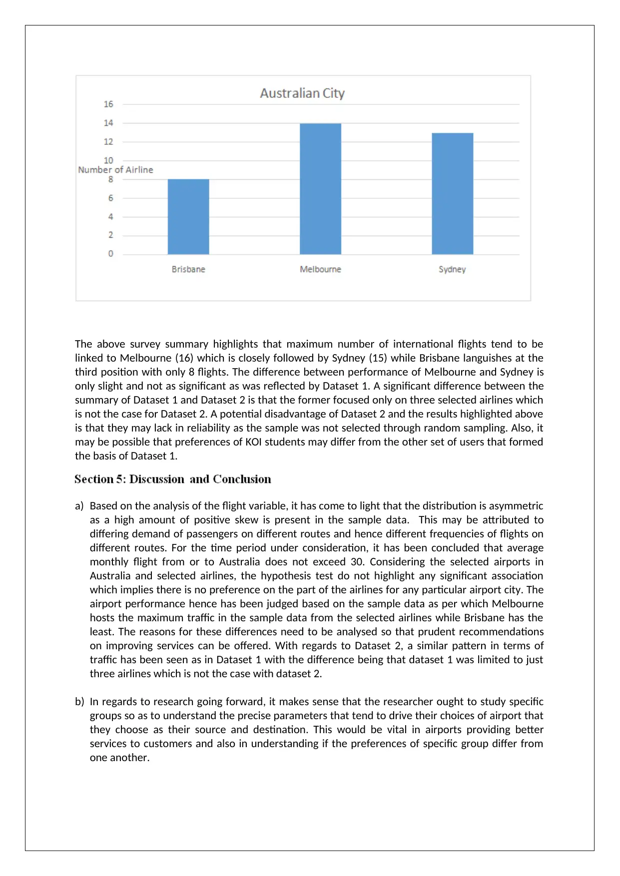
The above survey summary highlights that maximum number of international flights tend to be
linked to Melbourne (16) which is closely followed by Sydney (15) while Brisbane languishes at the
third position with only 8 flights. The difference between performance of Melbourne and Sydney is
only slight and not as significant as was reflected by Dataset 1. A significant difference between the
summary of Dataset 1 and Dataset 2 is that the former focused only on three selected airlines which
is not the case for Dataset 2. A potential disadvantage of Dataset 2 and the results highlighted above
is that they may lack in reliability as the sample was not selected through random sampling. Also, it
may be possible that preferences of KOI students may differ from the other set of users that formed
the basis of Dataset 1.
a) Based on the analysis of the flight variable, it has come to light that the distribution is asymmetric
as a high amount of positive skew is present in the sample data. This may be attributed to
differing demand of passengers on different routes and hence different frequencies of flights on
different routes. For the time period under consideration, it has been concluded that average
monthly flight from or to Australia does not exceed 30. Considering the selected airports in
Australia and selected airlines, the hypothesis test do not highlight any significant association
which implies there is no preference on the part of the airlines for any particular airport city. The
airport performance hence has been judged based on the sample data as per which Melbourne
hosts the maximum traffic in the sample data from the selected airlines while Brisbane has the
least. The reasons for these differences need to be analysed so that prudent recommendations
on improving services can be offered. With regards to Dataset 2, a similar pattern in terms of
traffic has been seen as in Dataset 1 with the difference being that dataset 1 was limited to just
three airlines which is not the case with dataset 2.
b) In regards to research going forward, it makes sense that the researcher ought to study specific
groups so as to understand the precise parameters that tend to drive their choices of airport that
they choose as their source and destination. This would be vital in airports providing better
services to customers and also in understanding if the preferences of specific group differ from
one another.
References
AnnaAero (2018) International airlines now carry 25% of Australian traffic; Sunshine Coast is flying in
terms of passenger growth; preparing for non-stop UK, [online] Available at
https://www.anna.aero/2018/02/27/international-airlines-now-carry-25-australian-traffic/[Assessed
January 11, 2019]
Fehr, F. H. and Grossman, G. (2013). An introduction to sets, probability and hypothesis testing. 3rd
ed. Ohio: Heath pp. 154-159.
Harmon, M. (2016) Hypothesis Testing in Excel - The Excel Statistical Master. 7th ed. Florida: Mark
Harmon pp 245-248.
Hastie, T., Tibshirani, R. and Friedman, J. (2014) The Elements of Statistical Learning. 4th ed. New
York: Springer Publications pp. 169-172.
Koch, K.R. (2013) Parameter Estimation and Hypothesis Testing in Linear Models. 2nd ed. London:
Springer Science & Business Media pp. 368-373.
Lehman, L. E. and Romano, P. J. (2016) Testing Statistical Hypotheses. 3rd ed. Berlin: Springer
Science & Business Media pp. 325-327.
⊘ This is a preview!⊘
Do you want full access?
Subscribe today to unlock all pages.
Trusted by 1+ million students worldwide
1 out of 9
Related Documents


Your All-in-One AI-Powered Toolkit for Academic Success.
+13062052269
info@desklib.com
Available 24*7 on WhatsApp / Email
![[object Object]](/_next/static/media/star-bottom.7253800d.svg)
Unlock your academic potential
Copyright © 2020–2026 A2Z Services. All Rights Reserved. Developed and managed by ZUCOL.