BUS708 - Statistical Modelling: Analyzing Gender Pay Gap in Australia
VerifiedAdded on 2023/06/12
|12
|2682
|199
Report
AI Summary
This report investigates gender pay disparities using statistical modeling and two datasets. The first dataset, sourced from the Australian Taxation Office, includes salary and occupation data. The second dataset, collected via questionnaires, provides additional insights. Summary statistics, including cross-tabulations and correlation analyses, reveal differences in gender representation across occupations and a weak positive correlation between gender and salary. Inferential statistics, such as t-tests, indicate a significant difference in mean salaries between males and females and a longer time for females to get promotions. The analysis confirms that gender-based preferences may influence hiring and remuneration practices. The full report is available on Desklib, where students can find similar solved assignments and past papers.

Research 1
Name
Tutor
Institution
Date
Name
Tutor
Institution
Date
Paraphrase This Document
Need a fresh take? Get an instant paraphrase of this document with our AI Paraphraser
Research 2
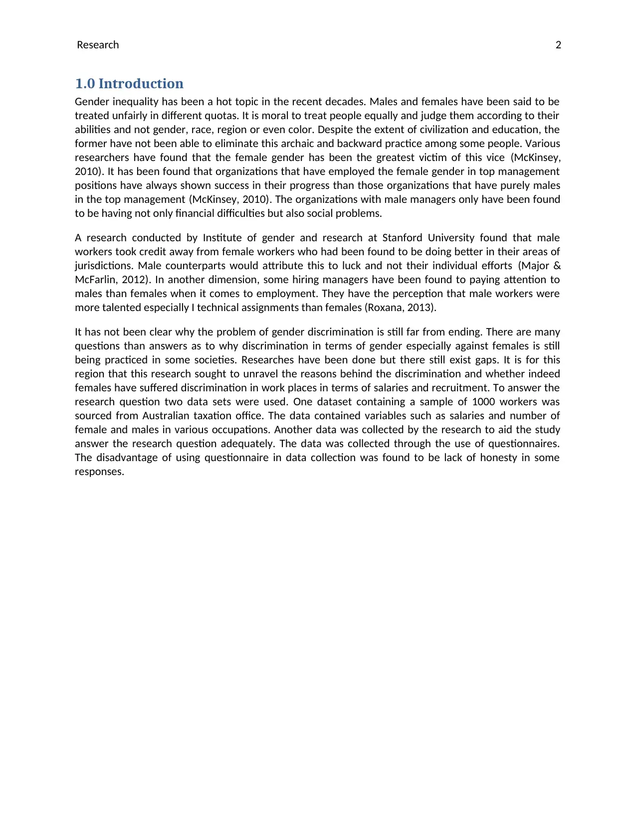
1.0 Introduction
Gender inequality has been a hot topic in the recent decades. Males and females have been said to be
treated unfairly in different quotas. It is moral to treat people equally and judge them according to their
abilities and not gender, race, region or even color. Despite the extent of civilization and education, the
former have not been able to eliminate this archaic and backward practice among some people. Various
researchers have found that the female gender has been the greatest victim of this vice (McKinsey,
2010). It has been found that organizations that have employed the female gender in top management
positions have always shown success in their progress than those organizations that have purely males
in the top management (McKinsey, 2010). The organizations with male managers only have been found
to be having not only financial difficulties but also social problems.
A research conducted by Institute of gender and research at Stanford University found that male
workers took credit away from female workers who had been found to be doing better in their areas of
jurisdictions. Male counterparts would attribute this to luck and not their individual efforts (Major &
McFarlin, 2012). In another dimension, some hiring managers have been found to paying attention to
males than females when it comes to employment. They have the perception that male workers were
more talented especially I technical assignments than females (Roxana, 2013).
It has not been clear why the problem of gender discrimination is still far from ending. There are many
questions than answers as to why discrimination in terms of gender especially against females is still
being practiced in some societies. Researches have been done but there still exist gaps. It is for this
region that this research sought to unravel the reasons behind the discrimination and whether indeed
females have suffered discrimination in work places in terms of salaries and recruitment. To answer the
research question two data sets were used. One dataset containing a sample of 1000 workers was
sourced from Australian taxation office. The data contained variables such as salaries and number of
female and males in various occupations. Another data was collected by the research to aid the study
answer the research question adequately. The data was collected through the use of questionnaires.
The disadvantage of using questionnaire in data collection was found to be lack of honesty in some
responses.
Research 3
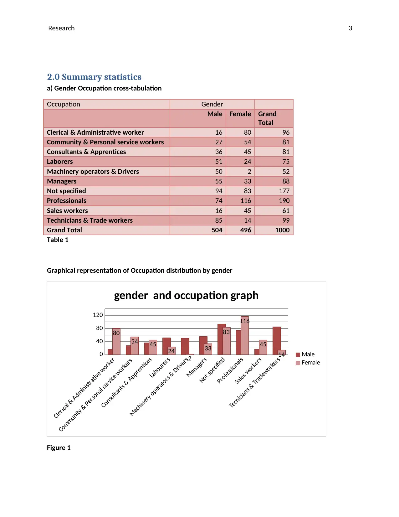
2.0 Summary statistics
a) Gender Occupation cross-tabulation
Occupation Gender
Male Female Grand
Total
Clerical & Administrative worker 16 80 96
Community & Personal service workers 27 54 81
Consultants & Apprentices 36 45 81
Laborers 51 24 75
Machinery operators & Drivers 50 2 52
Managers 55 33 88
Not specified 94 83 177
Professionals 74 116 190
Sales workers 16 45 61
Technicians & Trade workers 85 14 99
Grand Total 504 496 1000
Table 1
Graphical representation of Occupation distribution by gender
Clerical & Administrative worker
Community & Personal service workers
Consultants & Apprentices
Labourers
Machinery operators & Drivers
Managers
Not specified
Professionals
Sales workers
Tecnicians & Tradeworkers
0
40
80
120
80
54 45
24
2
33
83
116
45
14
gender and occupation graph
Male
Female
Figure 1
⊘ This is a preview!⊘
Do you want full access?
Subscribe today to unlock all pages.
Trusted by 1+ million students worldwide
Research 4
In order for the research to establish whether there were more males and females or vice versa, the
research decided to analyze the distribution of both gender by occupation. This analysis sought to find
the proportion of males and females in each profession to establish whether there are glaring
disparities. The graphical analysis above shows that out of the 10 professions, the proportion of males
was higher than that of females in 5 of them. The proportion of females was also high in the remaining 5
professions. For example the proportion of females was high in clerical and administrative jobs. They
were 80 while the males were 16. Their proportion was also high in community and personal service
jobs. Their number was 54 while the males were 27. The number of females was 45 and females were
16 among consultants and apprentices. Lastly, the number of females was also high among sales and
professional workers. Their number was 116 and 45 respectively while that of their counterparts was 74
and 16 respectively. The occupations where the males were the majority were among laborers, machine
operators, technicians and managers. Their number was 51, 50, 85 and 55 respectively. Their
counterparts in those professions were 24,2,33, 83 and 14 respectively.
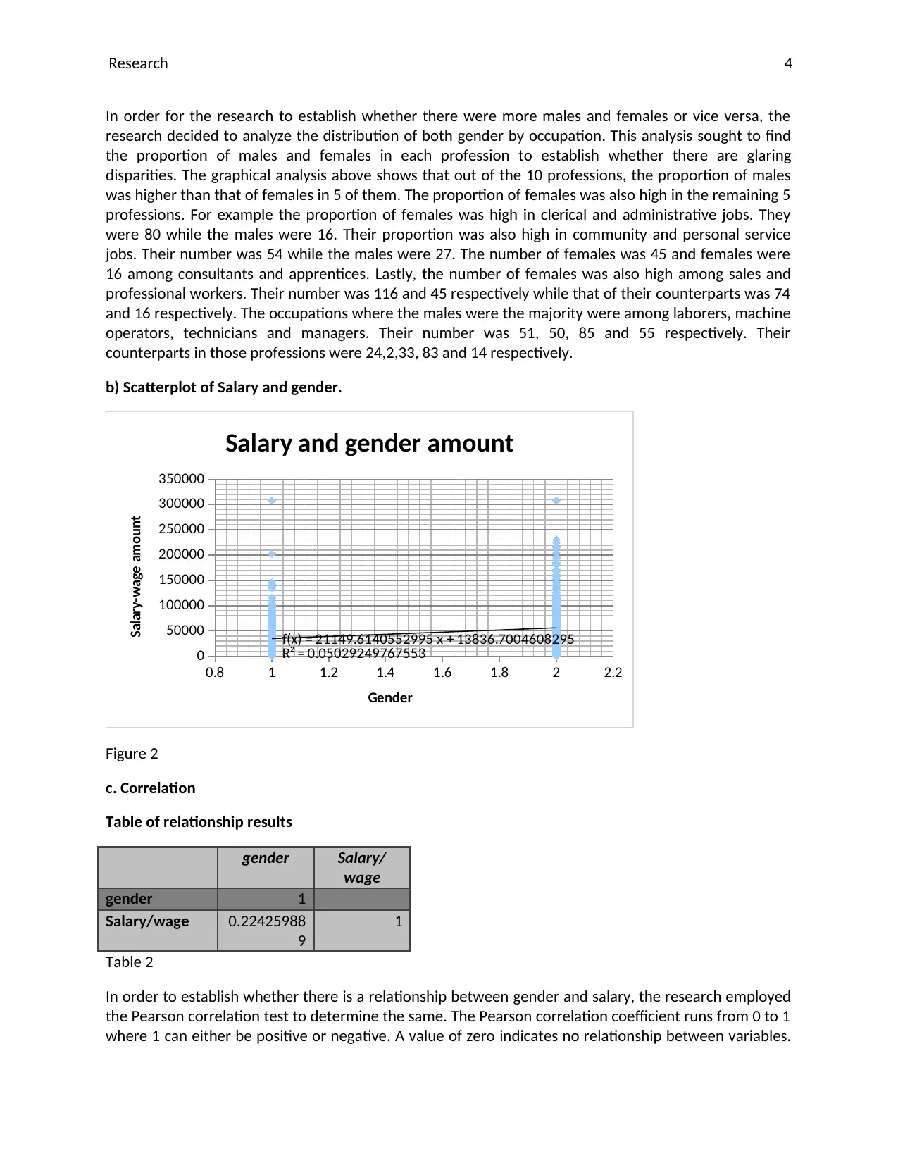
b) Scatterplot of Salary and gender.
0.8 1 1.2 1.4 1.6 1.8 2 2.2
0
50000
100000
150000
200000
250000
300000
350000
f(x) = 21149.6140552995 x + 13836.7004608295
R² = 0.05029249767553
Salary and gender amount
Gender
Salary-wage amount
Figure 2
c. Correlation
Table of relationship results
gender Salary/
wage
gender 1
Salary/wage 0.22425988
9
1
Table 2
In order to establish whether there is a relationship between gender and salary, the research employed
the Pearson correlation test to determine the same. The Pearson correlation coefficient runs from 0 to 1
where 1 can either be positive or negative. A value of zero indicates no relationship between variables.
In order for the research to establish whether there were more males and females or vice versa, the
research decided to analyze the distribution of both gender by occupation. This analysis sought to find
the proportion of males and females in each profession to establish whether there are glaring
disparities. The graphical analysis above shows that out of the 10 professions, the proportion of males
was higher than that of females in 5 of them. The proportion of females was also high in the remaining 5
professions. For example the proportion of females was high in clerical and administrative jobs. They
were 80 while the males were 16. Their proportion was also high in community and personal service
jobs. Their number was 54 while the males were 27. The number of females was 45 and females were
16 among consultants and apprentices. Lastly, the number of females was also high among sales and
professional workers. Their number was 116 and 45 respectively while that of their counterparts was 74
and 16 respectively. The occupations where the males were the majority were among laborers, machine
operators, technicians and managers. Their number was 51, 50, 85 and 55 respectively. Their
counterparts in those professions were 24,2,33, 83 and 14 respectively.
b) Scatterplot of Salary and gender.
0.8 1 1.2 1.4 1.6 1.8 2 2.2
0
50000
100000
150000
200000
250000
300000
350000
f(x) = 21149.6140552995 x + 13836.7004608295
R² = 0.05029249767553
Salary and gender amount
Gender
Salary-wage amount
Figure 2
c. Correlation
Table of relationship results
gender Salary/
wage
gender 1
Salary/wage 0.22425988
9
1
Table 2
In order to establish whether there is a relationship between gender and salary, the research employed
the Pearson correlation test to determine the same. The Pearson correlation coefficient runs from 0 to 1
where 1 can either be positive or negative. A value of zero indicates no relationship between variables.
Paraphrase This Document
Need a fresh take? Get an instant paraphrase of this document with our AI Paraphraser
Research 5
Correlation coefficient of 1 indicates a perfect strong positive correlation. Correlation coefficient of -1
indicates a perfect strong negative correlation. Having known that, the correlation coefficient between
above which is 0.22 indicates a weak but positive correlation between gender and salary.
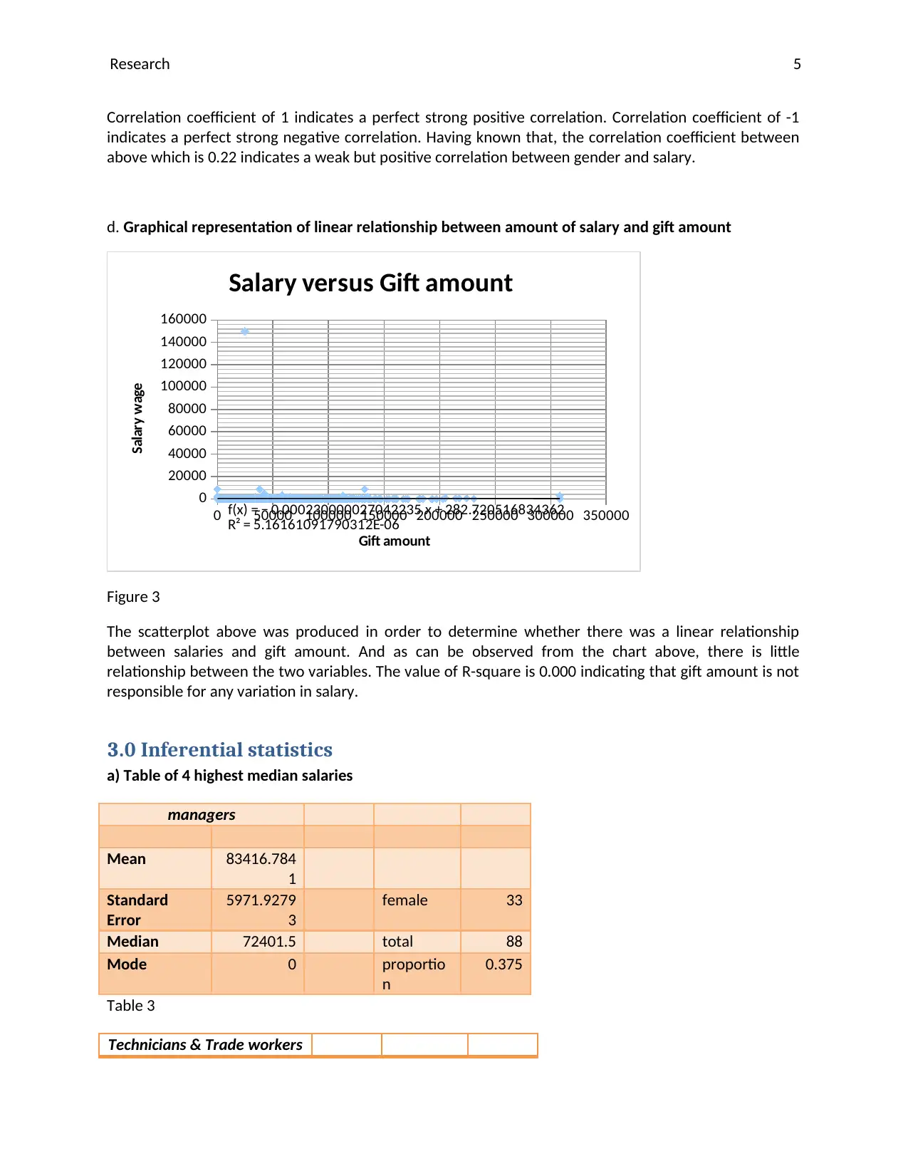
d. Graphical representation of linear relationship between amount of salary and gift amount
0 50000 100000 150000 200000 250000 300000 350000
0
20000
40000
60000
80000
100000
120000
140000
160000
f(x) = − 0.000230000027042235 x + 282.720516834362
R² = 5.16161091790312E-06
Salary versus Gift amount
Gift amount
Salary wage
Figure 3
The scatterplot above was produced in order to determine whether there was a linear relationship
between salaries and gift amount. And as can be observed from the chart above, there is little
relationship between the two variables. The value of R-square is 0.000 indicating that gift amount is not
responsible for any variation in salary.
3.0 Inferential statistics
a) Table of 4 highest median salaries
managers
Mean 83416.784
1
Standard
Error
5971.9279
3
female 33
Median 72401.5 total 88
Mode 0 proportio
n
0.375
Table 3
Technicians & Trade workers
Correlation coefficient of 1 indicates a perfect strong positive correlation. Correlation coefficient of -1
indicates a perfect strong negative correlation. Having known that, the correlation coefficient between
above which is 0.22 indicates a weak but positive correlation between gender and salary.
d. Graphical representation of linear relationship between amount of salary and gift amount
0 50000 100000 150000 200000 250000 300000 350000
0
20000
40000
60000
80000
100000
120000
140000
160000
f(x) = − 0.000230000027042235 x + 282.720516834362
R² = 5.16161091790312E-06
Salary versus Gift amount
Gift amount
Salary wage
Figure 3
The scatterplot above was produced in order to determine whether there was a linear relationship
between salaries and gift amount. And as can be observed from the chart above, there is little
relationship between the two variables. The value of R-square is 0.000 indicating that gift amount is not
responsible for any variation in salary.
3.0 Inferential statistics
a) Table of 4 highest median salaries
managers
Mean 83416.784
1
Standard
Error
5971.9279
3
female 33
Median 72401.5 total 88
Mode 0 proportio
n
0.375
Table 3
Technicians & Trade workers
Research 6
female 14
Mean 69624.4040
4
total 99
Standard
Error
4447.82987
4
proportio
n
0.14
Median 64886
Mode #N/A
Table 4
Professional
Mean 69771.03158
Standard Error 3843.825377 female 116
Median 62108 total 190
Mode 308183 proportio
n
0.61
Table 5
Clerical & Administrative
worker
Mean 46762.51
Standard Error 4163.464 female 80
Median 41605 total 96
Mode #N/A proportio
n
0.83
Table 6
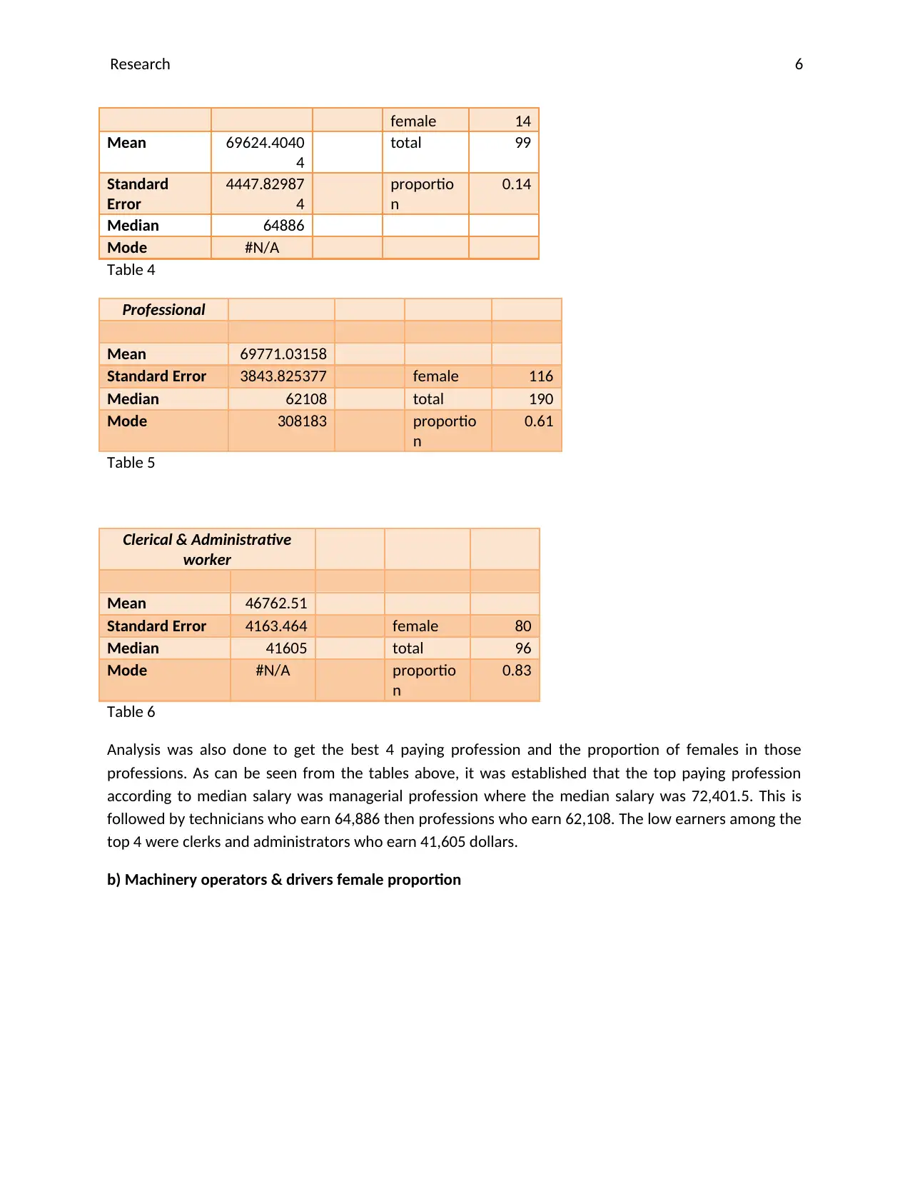
Analysis was also done to get the best 4 paying profession and the proportion of females in those
professions. As can be seen from the tables above, it was established that the top paying profession
according to median salary was managerial profession where the median salary was 72,401.5. This is
followed by technicians who earn 64,886 then professions who earn 62,108. The low earners among the
top 4 were clerks and administrators who earn 41,605 dollars.
b) Machinery operators & drivers female proportion
female 14
Mean 69624.4040
4
total 99
Standard
Error
4447.82987
4
proportio
n
0.14
Median 64886
Mode #N/A
Table 4
Professional
Mean 69771.03158
Standard Error 3843.825377 female 116
Median 62108 total 190
Mode 308183 proportio
n
0.61
Table 5
Clerical & Administrative
worker
Mean 46762.51
Standard Error 4163.464 female 80
Median 41605 total 96
Mode #N/A proportio
n
0.83
Table 6
Analysis was also done to get the best 4 paying profession and the proportion of females in those
professions. As can be seen from the tables above, it was established that the top paying profession
according to median salary was managerial profession where the median salary was 72,401.5. This is
followed by technicians who earn 64,886 then professions who earn 62,108. The low earners among the
top 4 were clerks and administrators who earn 41,605 dollars.
b) Machinery operators & drivers female proportion
⊘ This is a preview!⊘
Do you want full access?
Subscribe today to unlock all pages.
Trusted by 1+ million students worldwide
Research 7
Table 7
Hypothesis testing
H0: ῥ = 80%
Versus
H0: ῥ > 80%
Z−value= ῥ− p
√ p .q
n
Z−value= 0.8−0.6
√ 0.2× 0.8
127
=1.69
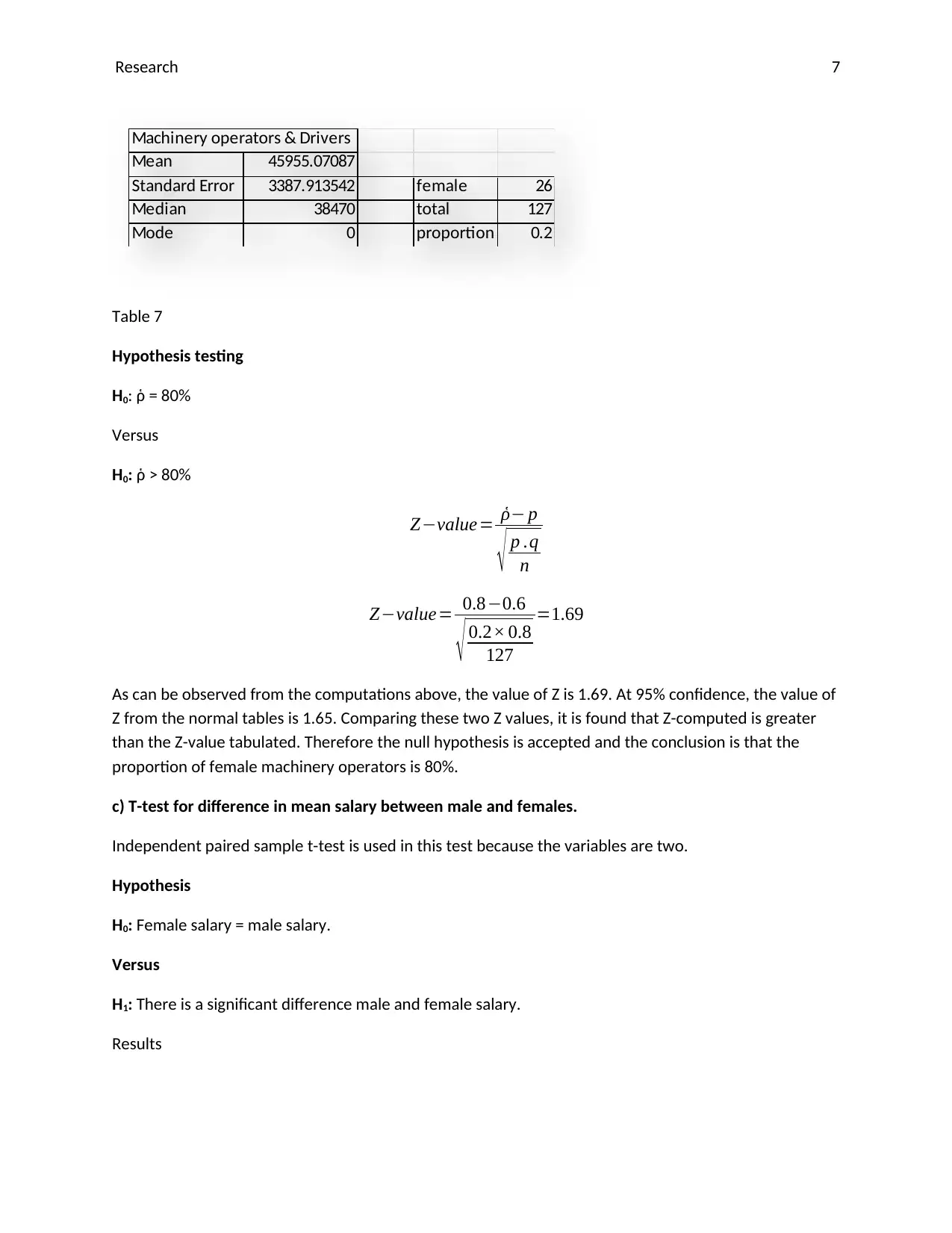
As can be observed from the computations above, the value of Z is 1.69. At 95% confidence, the value of
Z from the normal tables is 1.65. Comparing these two Z values, it is found that Z-computed is greater
than the Z-value tabulated. Therefore the null hypothesis is accepted and the conclusion is that the
proportion of female machinery operators is 80%.
c) T-test for difference in mean salary between male and females.
Independent paired sample t-test is used in this test because the variables are two.
Hypothesis
H0: Female salary = male salary.
Versus
H1: There is a significant difference male and female salary.
Results
Machinery operators & Drivers
Mean 45955.07087
Standard Error 3387.913542 female 26
Median 38470 total 127
Mode 0 proportion 0.2
Table 7
Hypothesis testing
H0: ῥ = 80%
Versus
H0: ῥ > 80%
Z−value= ῥ− p
√ p .q
n
Z−value= 0.8−0.6
√ 0.2× 0.8
127
=1.69
As can be observed from the computations above, the value of Z is 1.69. At 95% confidence, the value of
Z from the normal tables is 1.65. Comparing these two Z values, it is found that Z-computed is greater
than the Z-value tabulated. Therefore the null hypothesis is accepted and the conclusion is that the
proportion of female machinery operators is 80%.
c) T-test for difference in mean salary between male and females.
Independent paired sample t-test is used in this test because the variables are two.
Hypothesis
H0: Female salary = male salary.
Versus
H1: There is a significant difference male and female salary.
Results
Machinery operators & Drivers
Mean 45955.07087
Standard Error 3387.913542 female 26
Median 38470 total 127
Mode 0 proportion 0.2
Paraphrase This Document
Need a fresh take? Get an instant paraphrase of this document with our AI Paraphraser
Research 8
Table 8
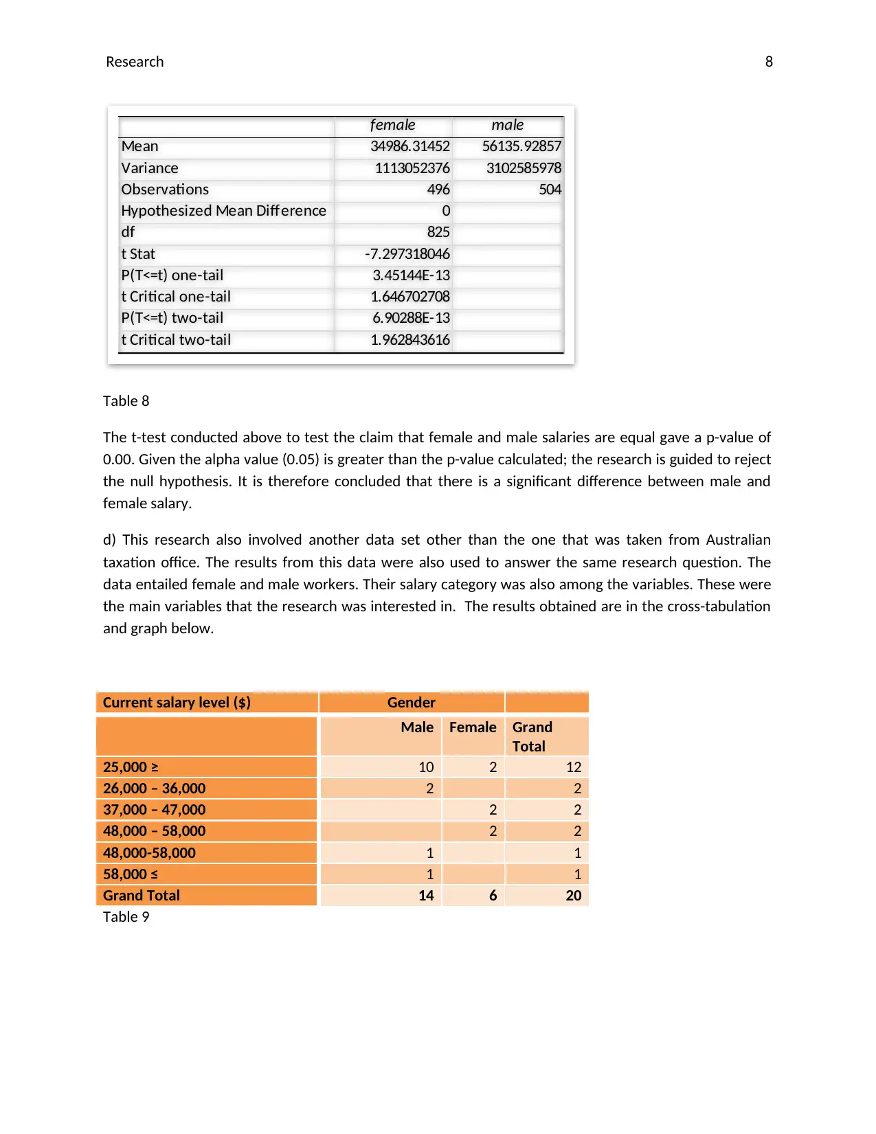
The t-test conducted above to test the claim that female and male salaries are equal gave a p-value of
0.00. Given the alpha value (0.05) is greater than the p-value calculated; the research is guided to reject
the null hypothesis. It is therefore concluded that there is a significant difference between male and
female salary.
d) This research also involved another data set other than the one that was taken from Australian
taxation office. The results from this data were also used to answer the same research question. The
data entailed female and male workers. Their salary category was also among the variables. These were
the main variables that the research was interested in. The results obtained are in the cross-tabulation
and graph below.
Current salary level ($) Gender
Male Female Grand
Total
25,000 ≥ 10 2 12
26,000 – 36,000 2 2
37,000 – 47,000 2 2
48,000 – 58,000 2 2
48,000-58,000 1 1
58,000 ≤ 1 1
Grand Total 14 6 20
Table 9
female male
Mean 34986.31452 56135.92857
Variance 1113052376 3102585978
Observations 496 504
Hypothesized Mean Difference 0
df 825
t Stat -7.297318046
P(T<=t) one-tail 3.45144E-13
t Critical one-tail 1.646702708
P(T<=t) two-tail 6.90288E-13
t Critical two-tail 1.962843616
Table 8
The t-test conducted above to test the claim that female and male salaries are equal gave a p-value of
0.00. Given the alpha value (0.05) is greater than the p-value calculated; the research is guided to reject
the null hypothesis. It is therefore concluded that there is a significant difference between male and
female salary.
d) This research also involved another data set other than the one that was taken from Australian
taxation office. The results from this data were also used to answer the same research question. The
data entailed female and male workers. Their salary category was also among the variables. These were
the main variables that the research was interested in. The results obtained are in the cross-tabulation
and graph below.
Current salary level ($) Gender
Male Female Grand
Total
25,000 ≥ 10 2 12
26,000 – 36,000 2 2
37,000 – 47,000 2 2
48,000 – 58,000 2 2
48,000-58,000 1 1
58,000 ≤ 1 1
Grand Total 14 6 20
Table 9
female male
Mean 34986.31452 56135.92857
Variance 1113052376 3102585978
Observations 496 504
Hypothesized Mean Difference 0
df 825
t Stat -7.297318046
P(T<=t) one-tail 3.45144E-13
t Critical one-tail 1.646702708
P(T<=t) two-tail 6.90288E-13
t Critical two-tail 1.962843616
Research 9
25,000 ≥ 26,000 –
36,000 37,000 –
47,000 48,000 –
58,000 48,000-
58,000 58,000 ≤
0
2
4
6
8
10
12
Male
Female
Figure 4
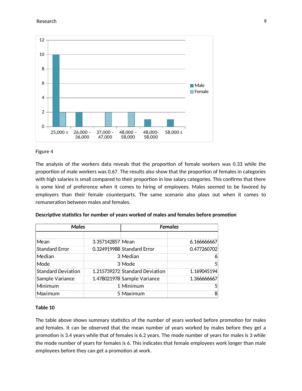
The analysis of the workers data reveals that the proportion of female workers was 0.33 while the
proportion of male workers was 0.67. The results also show that the proportion of females in categories
with high salaries is small compared to their proportion in low salary categories. This confirms that there
is some kind of preference when it comes to hiring of employees. Males seemed to be favored by
employers than their female counterparts. The same scenario also plays out when it comes to
remuneration between males and females.
Descriptive statistics for number of years worked of males and females before promotion
Mean 3.357142857 Mean 6.166666667
Standard Error 0.324919988 Standard Error 0.477260702
Median 3 Median 6
Mode 3 Mode 5
Standard Deviation 1.215739272 Standard Deviation 1.169045194
Sample Variance 1.478021978 Sample Variance 1.366666667
Minimum 1 Minimum 5
Maximum 5 Maximum 8
Males Females
Table 10
The table above shows summary statistics of the number of years worked before promotion for males
and females. It can be observed that the mean number of years worked by males before they get a
promotion is 3.4 years while that of females is 6.2 years. The mode number of years for males is 3 while
the mode number of years for females is 6. This indicates that female employees work longer than male
employees before they can get a promotion at work.
25,000 ≥ 26,000 –
36,000 37,000 –
47,000 48,000 –
58,000 48,000-
58,000 58,000 ≤
0
2
4
6
8
10
12
Male
Female
Figure 4
The analysis of the workers data reveals that the proportion of female workers was 0.33 while the
proportion of male workers was 0.67. The results also show that the proportion of females in categories
with high salaries is small compared to their proportion in low salary categories. This confirms that there
is some kind of preference when it comes to hiring of employees. Males seemed to be favored by
employers than their female counterparts. The same scenario also plays out when it comes to
remuneration between males and females.
Descriptive statistics for number of years worked of males and females before promotion
Mean 3.357142857 Mean 6.166666667
Standard Error 0.324919988 Standard Error 0.477260702
Median 3 Median 6
Mode 3 Mode 5
Standard Deviation 1.215739272 Standard Deviation 1.169045194
Sample Variance 1.478021978 Sample Variance 1.366666667
Minimum 1 Minimum 5
Maximum 5 Maximum 8
Males Females
Table 10
The table above shows summary statistics of the number of years worked before promotion for males
and females. It can be observed that the mean number of years worked by males before they get a
promotion is 3.4 years while that of females is 6.2 years. The mode number of years for males is 3 while
the mode number of years for females is 6. This indicates that female employees work longer than male
employees before they can get a promotion at work.
⊘ This is a preview!⊘
Do you want full access?
Subscribe today to unlock all pages.
Trusted by 1+ million students worldwide
Research
10
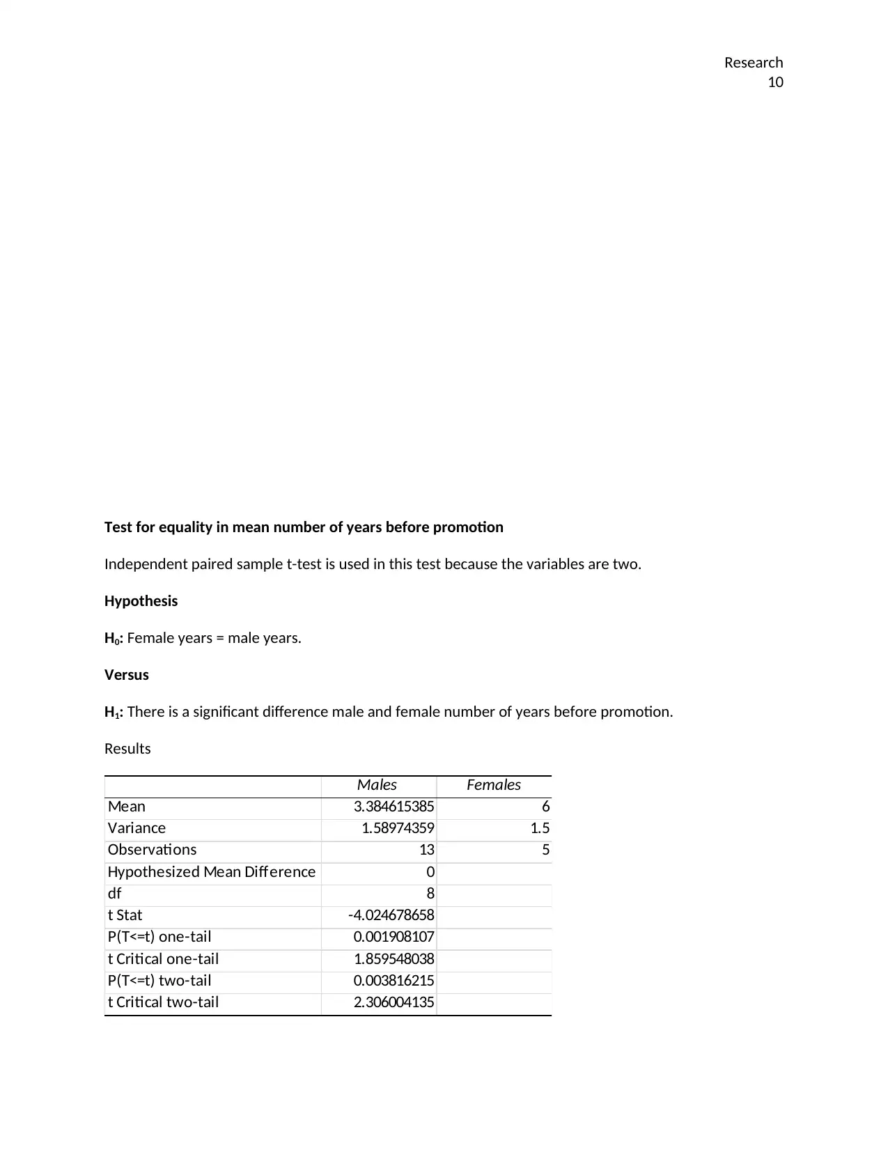
Test for equality in mean number of years before promotion
Independent paired sample t-test is used in this test because the variables are two.
Hypothesis
H0: Female years = male years.
Versus
H1: There is a significant difference male and female number of years before promotion.
Results
Males Females
Mean 3.384615385 6
Variance 1.58974359 1.5
Observations 13 5
Hypothesized Mean Difference 0
df 8
t Stat -4.024678658
P(T<=t) one-tail 0.001908107
t Critical one-tail 1.859548038
P(T<=t) two-tail 0.003816215
t Critical two-tail 2.306004135
10
Test for equality in mean number of years before promotion
Independent paired sample t-test is used in this test because the variables are two.
Hypothesis
H0: Female years = male years.
Versus
H1: There is a significant difference male and female number of years before promotion.
Results
Males Females
Mean 3.384615385 6
Variance 1.58974359 1.5
Observations 13 5
Hypothesized Mean Difference 0
df 8
t Stat -4.024678658
P(T<=t) one-tail 0.001908107
t Critical one-tail 1.859548038
P(T<=t) two-tail 0.003816215
t Critical two-tail 2.306004135
Paraphrase This Document
Need a fresh take? Get an instant paraphrase of this document with our AI Paraphraser
Research
11
Table 11
The t-test conducted above to test the claim that female and male employees’ number of working years
before promotion is equal gave a p-value of 0.00. Given the alpha value (0.05) is greater than the p-
value calculated; the research is guided to reject the null hypothesis. It is therefore concluded that there
is a significant difference between male and female number of working years before promotion.
4.0 Discussion and conclusion
This research study has come up with various findings that has enabled it make various inferences which
has enabled the research to answer its main question. It was hypothesized earlier that the female
gender had been discriminated in work places when it came to salaries and also employment. The first
data showed that there was some balance between males and females when it came to proportions in
each profession. Out of the 10 professions, the proportion of males was higher than that of females in 5
of them. The proportion of females was also high in the remaining 5 professions. For example the
proportion of females was high in clerical and administrative jobs. They were 80 while the males were
16. Their proportion was also high in community and personal service jobs. Their number was 54 while
the males were 27. The number of females was 45 and females were 16 among consultants and
apprentices. Lastly, the number of females was also high among sales and professional workers. Their
number was 116 and 45 respectively while that of their counterparts was 74 and 16 respectively. The
occupations where the males were the majority were among laborers, machine operators, technicians
and managers. Their number was 51, 50, 85 and 55 respectively. Their counterparts in those professions
were 24,2,33, 83 and 14 respectively. However, the second data found that there was inequality in
employment where the proportion of females was much lower than the proportion of males. To add on,
the number of years that male employees worked before they were awarded a promotion were less
compared to the number of years worked by female employees before being awarded with a
promotion. Since this research concentrated on the employee side, it is not enough to make conclusions
with finality. Employers’ side of the story should also be incorporated in such a research in order to
make valid conclusions. This means that there is still a gap in this research, therefore this research study
recommend further research on employers so as to adequately answer the research question.
Research
12
References
Major, B., & McFarlin, D. B. (2012). Overworked and underpaid: On the Nature of Gender Differences in
Personal Entitlement. Journal of Personality and Social Psychology, 47(6), 44-56.
McKinsey, C. (2010). Women Matter:Gender Diversity; A Corporate Performance Driver.
Roxana , B. (2013). Women in the workplace: A research round up.
⊘ This is a preview!⊘
Do you want full access?
Subscribe today to unlock all pages.
Trusted by 1+ million students worldwide
1 out of 12
Related Documents


Your All-in-One AI-Powered Toolkit for Academic Success.
+13062052269
info@desklib.com
Available 24*7 on WhatsApp / Email
![[object Object]](/_next/static/media/star-bottom.7253800d.svg)
Unlock your academic potential
Copyright © 2020–2026 A2Z Services. All Rights Reserved. Developed and managed by ZUCOL.