Report on Business Decision Analysis, Pricing and CVP Analysis

This report provides a comprehensive analysis of decision-making processes, incorporating utility functions, standard gamble assessments, and various decision criteria such as optimistic, pessimistic, and regret approaches. It delves into expected monetary value (EMV) calculations, including the expected value of perfect information (EVPI), and explores the value of information through conditional probabilities and Bayesian analysis. The report also covers Monte Carlo simulation for profit forecasting and includes a section on regression analysis to determine overhead costs based on machine hours and batch sizes. Furthermore, it examines cost-volume-profit (CVP) analysis to assess break-even points and profit targets under different pricing scenarios. The analysis is supported by calculations, decision trees, and tables to illustrate key concepts and findings.

Contents
Decision Analysis............................................................................................................................2
Q1a...............................................................................................................................................2
Q1b...............................................................................................................................................3
Q1b1.........................................................................................................................................3
Q1b2.........................................................................................................................................3
Q1b3.........................................................................................................................................4
Q1b4.........................................................................................................................................4
Q1b5.........................................................................................................................................5
Q1b6.........................................................................................................................................5
Value of information........................................................................................................................6
Q2a...............................................................................................................................................6
Q2b...............................................................................................................................................7
Q1c...............................................................................................................................................7
Q1d...............................................................................................................................................8
Monte Carlo Simulation................................................................................................................12
Q3a.............................................................................................................................................12
Q3b.............................................................................................................................................12
Q3c.............................................................................................................................................13
New Pricing Strategy - Report...............................................................................................13
Regression Analysis.......................................................................................................................15
Q4a.............................................................................................................................................15
Q4b.............................................................................................................................................15
1 – Overhead cost vs Machine Hours.................................................................................16
3 – Overhead VS Machine hours + Batches.......................................................................17
Q4c.............................................................................................................................................17
Q4d.............................................................................................................................................18
CVP Analysis.................................................................................................................................18
Q5a.............................................................................................................................................18
Q5b.............................................................................................................................................19
Q5c.............................................................................................................................................19
Q5d.............................................................................................................................................19

Q5d1...........................................................................................................................................19
Q5d2...........................................................................................................................................19
References:....................................................................................................................................20

Decision Analysis
Q1a
Discuss how a utility function can be assessed. What is a standard gamble and how is it used
in determining utility values?
To assess a given Decision, the monetary value outcome of single decision choices made should
be normalized with the risk involved with the decision. In a decision choice after considering the
risk attached to it, the numeric representation is given by the Utility function.
Assessing utility function scenario consider the Decision as a gamble and alternative 1 with only
2 possible outcome, 0 as utility for worst outcome stat 1 and 1 to best outcome state 2. p & q are
probabilities involved. Then, q = 1-p
Finding utility for any other scenario, we consider Alternative 2 with worst and best outcome.
When we equate Alternative 1 and alternative 2 outcomes, then;
Utility of Alternative1
p(1)+(1−p)(0)=p
 Utility of Alternative 2=x
 Utility of Alternative 2(x)=Utility of Alternative 1= p
x= p
We can therefore assign utility value of any other outcome using the summary below
Below Decision stump summarizes the Standard gamble.
.

Q1b
Below are details of Barnes, Decision outcomes.
 Amount of Total Investment = 10000
 Investment option1 – share Market
Good return = 14%
Fair return = 8%
Bad return = 0%
 Investment option2 – Government bonds
Constant = 9%
Q1b1
The table below shows Decision Matrix of the the above values;
Decision matrix
Investment option
Share market Government bonds
Market
conditions
Good 1400 900
Fair 800 900
Bad 0 900
Q1b2
Which alternative would an optimist choose?
Optimist will go for maximum choice out of the maximum outcome on each of the market state.
Maximax-Optimist choice
Investment option Maximum
Share market Government bonds
Market
conditions
Good 1400 900 1400
Fair 800 900 900
Bad 0 900 900
Under optimistic criterion, the optimist choose, Share market as investment option.

Q1b3
Which alternative would a pessimist choose?
Pessimist will go for minimum choice among the minimum outcome in each market state.
Minimini-pessimist choice
Investment option Minimum
Share market Government bonds
Market
conditions
Good 1400 900 900
Fair 800 900 800
Bad 0 900 0
Under Pessimistic criterion, the pessimist will choose, Share market as investment option, with 0
return.
Q1b4
Which alternative is indicated by the criterion of regret?
Regret Criterion is given by the minimax opportunity loss state, where Opportunity loss for a
given state is the different between the state outcome and maximum outcome of a market state.
Example: Opportunity Loss for Government bonds in Good market state is;
1400(maximum of outcome for good market ) – 900( outcome of Govt bonds∈Good market )
¿ 500
Criterion for regret is state where opportunity loss is minimum, which is investment in
government bonds in good market state.

Investment option Max per state
Share market Government
bonds
State of market Good 1400 900 1400
Fair 800 900 900
Bad 0 900 900
Opportunity loss matrix
Share market Government
bond
Good 0 500
Fair 100 0
Bad 900 0
Maximum
opportunity loss
per option
900 500
Q1b5
Assuming probability of a good market = 0.4, a fair market = 0.4 and a bad market = 0.2, using
Expected monetary values what is the optimum action?
Probability per
market state
Investment option
Share market Government bond
Market
state
Good 0.4 1400 900
Fair 0.4 800 900
Bad 0.2 0 900
EMV =∑ total of Probability of market state∧outcomes attached .
EMV ( share market )=0.4 ×1400+0.4 × 800+0.2 ×0=880
EMV (Government bonds)=0.4 ×900+ 0.4 ×900+ 0.2× 900=900
Hence Optimum action would be investing in Government bonds.
Q1b6
What is the expected value of perfect information?
Expected Value with perfect Information is weighted average of maximum possible state of
available options and probability of occurrence of each state.
Thus;
EVwPI =0.4 × 1400+0.4 × 900+0.2 ×900=1100

Probability per
market state
Investment option Max in
state of
market
Share market Government
bond
Market state Good 0.4 1400 900 1400
Fair 0.4 800 900 900
Bad 0.2 0 900 900
Expected monetary value 1100
Expected value of Perfect Information is difference between the EVwPI and maximum of EVM
(900)
EVPI=1100 – 900=$ 200
Thus;
Expected value of Perfect Information is $200 for the given market state and investment options.
Value of information
 let P(FM) be the Probability for Market is Favorable.
 let P(UM) be the Probability for Market is Unfavorable.
 let P(FR|FM) be the probability for Research Favorable Given Market is Favorable.
 let P(UR|FM) be the probability for Research Unfavorable Given Market is Favorable.
 let P(UR|UM) be the probability for Research Unfavorable Given Market is Unfavorable.
 let P(FR|UM) be the probability for Research Favorable Given Market is Unfavorable.
 let P(FM|FR) be the Probability for Favorable Market given favorable Research
 let P(UM|FR) be the Probability for Unfavorable Market given favorable Research
 let P(FM|UR) be the Probability for favorable Market given Research Unfavorable.
 let P(UM|UR) be the Probability for Unfavorable Market given Research Unfavorable.
 let P(FR be the Probability for Favorable research
 let P(UR) be the Probability for unfavorable research
For a Razor Factory, If the market were favorable return is of $100,000, but if the market were
unfavorable loss is $60,000. Jim estimates the probability of a favorable market is 0.5
So, P( FM )=0.5∧P(UM )=0.5∧R (FM )=100000∧R (UM )=−$ 60000

Q2a
What should Jerry do? Show calculations
Jerry should calculate Estimated Monetary Value is either of the market conditions for either of
the 2 options, go for production or not go for production.
EMV is best of each condition weighted averaged against probability of occurrence for
condition.
EMV production={ R(FM )× P( FM )+ R( UM )× P (UM )}
EMV production=(0.5 ×100000+0.5 ×(−60000))
EMV production=20000
EMV no production={R(FM )× P( FM )+ R (UM )× P (UM )}
EMV no production=(0.5 × 0+0.5 ×0)
EMV no production=0
Option evaluation is best of EMV of either of 2 options. Which is corresponding to go for
production. Hence Jerry should go for Production.
Q2b
Revise the prior probabilities in light of his friend’s track record.
70% of friend’s past record is the time he would correctly provide a favorable market prediction
and 20% of the time he would incorrectly provide a favorable market prediction.
Prior Probabilities are prior probabilities for Favorable or unfavorable market conditions.
P( FM )=0.5
P(UM )=1 – P ( FM )=0.5
Q1c
What is the posterior probability of a good market given that his friend has provided an
unfavorable market prediction?
Posterior Probabilities, for Favorable Market given Favorable Research be P(FM|FR) and for
Unfavorable Market given Favorable Research be P(UM|FR).
To Calculate the Posterior Probabilities, Conditional Probabilities for P(FR|FM) and P(FR|UM)
is required.
As per friend’s track record.
P( FR∨FM )=0.7

P( FR∨UM )=0.2 .
Posterior probability Calculations for Favorable Research
State of
events
Prior Conditiona
l
probability
Joint Posterior
Favorable
market
P(FM)=0.5 P(FR|
FM)=0.7
P(FR ∩FM)= P(FR|FM)×P(FM)=0.35 0.78
Unfavorabl
e market
P(UM)=0.
5
P(FR|
UM)=0.2
P(FR ∩UM)= P(FR|UM)×P(FM)=0.10 0.22
Probability of favorable research
P(FR)=0.45
Joint Probability for Favorable market and Favorable Research P(FR∩FM) is product of P(FR|
FM) and P(FM) as calculated above = 0.35
While, Joint Probability for unfavorable market and Favorable Research P(FR∩UM) is product
of P(FR|UM) and P(UM) as calculated above =0.10
Taking sum of P(FR∩FM) and P(FR∩UM) gives the absolute probability for a favorable
research, which is P(FR) = 0.45.
The Bayes Theorem−P( A∨B)× P (B)=P (B∨ A)× P( A)
Hence ,
P( FM ∨FR)=P( FR∨FM ) × P( FM )/P(FR)=P (FR ∩ FM )/P(FR)=0.35 ÷ 0.45=0.78
P(UM ∨FR)=P(FR∨UM ) × P(UM )/ P( FR)=P(FR ∩ FM )/ P(FR)=0.10 ÷ 0.45=0.22
Q1d
What is the expected net gain or loss from engaging his friend to conduct the market
research? Should his friend be engaged? Why?
Expected Gain or loss for engaging the Friend for research can be calculated using a decision
tree.
Let P1 through P11 represent decision stumps in the Decision tree, while N1 to N9 represent the
outcome leaf nodes.
Let

P1 Represents decision node for Research∨do not conduct Research .
P2 Represents decision node for go for Production∨not go for Production .
P3 represents decision node for Research Favorable∨Unfavorable.
P4 represents decision node for Favorable Market ∨Unfavorable Market .
P5 isa dummy decision node for no production .
P6 represents decision node for go for Production∨not go for Production .
P7 represents decision node for go for Production∨not go for Production .
P8 represents decision node for Favorable Market∨Unfavorable Market .
P9 is a dummy decision node for no production .
P10 represents decision node for Favorable Market ∨Unfavorable Market
P11 is a dummy decision node for no production.
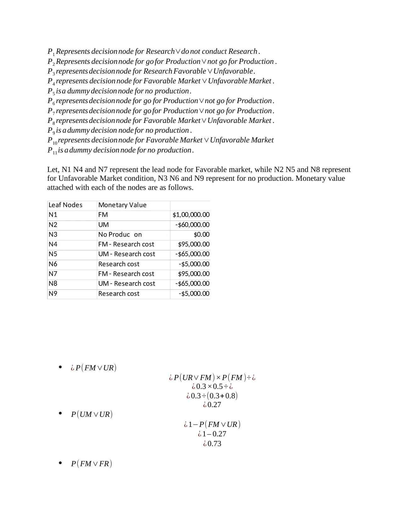
Let, N1 N4 and N7 represent the lead node for Favorable market, while N2 N5 and N8 represent
for Unfavorable Market condition, N3 N6 and N9 represent for no production. Monetary value
attached with each of the nodes are as follows.
eaf odesL N Monetary Value
N1 MF $1,00,000.00
N2 MU -$60,000.00
N3 o roducti onN P $0.00
N4 M Research costF - $95,000.00
N5 M Research costU - -$65,000.00
N6 Research cost -$5,000.00
N7 M Research costF - $95,000.00
N8 M Research costU - -$65,000.00
N9 Research cost -$5,000.00
 ¿ P(FM ∨UR)
¿ P(UR∨FM ) × P(FM )÷ ¿
¿ 0.3 ×0.5 ÷ ¿
¿ 0.3 ÷(0.3+ 0.8)
¿ 0.27
 P(UM ∨UR)
¿ 1−P(FM ∨UR )
¿ 1 – 0.27
¿ 0.73
 P(FM ∨FR)

¿ P( FR∨FM )× P(FM )/((P ( FR∨UM )× P(UM ))+( P( FR∨FM )∗P(FM )))
¿( 0.7 ×0.5)÷ (0.7 ×0.5+ 0.2× 0.5)
¿ 0.7 ÷ 0.9
¿ 0.78
 P(UM ∨FR)
¿ 1−P(FM ∨FR)
¿ 1 – 0.78
¿ 0.22
 P(FR)
As per Bayes theorem for conditional probability explained above , we have−¿
P( FR∨FM )× P (FM )=P(FM ∨FR)× P ( FR)
¿ ¿
¿(0.7 ×0.5)÷ 0.78
¿ 0.45
 P(UR )
¿ 1 – P(FR)
Conditional Probability values for different events summarized below are as follows.
robability ValuesP
MP(F ) 0.5
MP(U ) 0.5
R MP(F |F ) 0.7
R MP(U |F ) 0.3
R MP(U |U ) 0.8
R MP(F |U ) 0.2
M RP(F |F ) 0.78
M RP(U |F ) 0.22
M RP(F |U ) 0.27
M RP(U |U ) 0.72
RP(F ) 0.45
RP(U ) 0.55
Plotting the above information on a decision tree, as per below diagram.

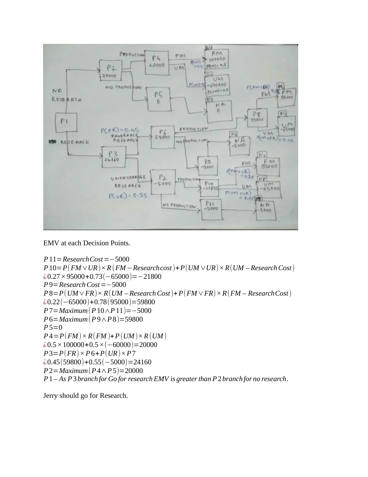
EMV at each Decision Points.
P 11=ResearchCost =−5000
P 10=P( FM ∨UR )× R ( FM −Researchcost )+ P(UM ∨UR)× R(UM – Research Cost )
¿ 0.27 × 95000+0.73(−65000)=−21800
P 9=Research Cost =−5000
P 8=P(UM∨FR)× R(UM – Research Cost )+ P(FM ∨FR)× R(FM – ResearchCost )
¿ 0.22(−65000)+0.78(95000)=59800
P 7=Maximum(P 10∧P 11)=−5000
P 6=Maximum(P 9∧P 8)=59800
P 5=0
P 4=P(FM )× R( FM )+P (UM )× R (UM )
¿ 0.5 ×100000+0.5 ×(−60000)=20000
P 3=P(FR)× P 6+ P(UR )× P 7
¿ 0.45(59800)+0.55(−5000)=24160
P 2=Maximum( P 4∧P 5)=20000
P 1 – As P 3 branch for Go for research EMV is greater than P 2 branch for no research.
Jerry should go for Research.

Monte Carlo Simulation
Q3a
MODEL
Month RN1 Demand Selling Price RN2 Profit Margin Fixed Costs Profit
1 =RAND() =VLOOKUP(B3,Q
3_Data!
$C$10:$D$16,2)
=RANDBETWEEN(Q
3_Data!B2,Q3_Data!
C2)
=RAND() =Q3_Data!$B$4 +
(E3*(Q3_Data!
$C$4 - Q3_Data!
$B$4))
2000 =C3*D3*F3-
G3
=A3+1 =TABLE(,J8) =TABLE(,J8) =TABLE(,J8) =TABLE(,J
8)
=TABLE(,J8) =TABLE(,J
8)
=TABLE(,J8)
=A4+1 =TABLE(,J8) =TABLE(,J8) =TABLE(,J8) =TABLE(,J
8)
=TABLE(,J8) =TABLE(,J
8)
=TABLE(,J8)
=A5+1 =TABLE(,J8) =TABLE(,J8) =TABLE(,J8) =TABLE(,J
8)
=TABLE(,J8) =TABLE(,J
8)
=TABLE(,J8)
=A6+1 =TABLE(,J8) =TABLE(,J8) =TABLE(,J8) =TABLE(,J
8)
=TABLE(,J8) =TABLE(,J
8)
=TABLE(,J8)
=A7+1 =TABLE(,J8) =TABLE(,J8) =TABLE(,J8) =TABLE(,J
8)
=TABLE(,J8) =TABLE(,J
8)
=TABLE(,J8)
=A8+1 =TABLE(,J8) =TABLE(,J8) =TABLE(,J8) =TABLE(,J
8)
=TABLE(,J8) =TABLE(,J
8)
=TABLE(,J8)
=A9+1 =TABLE(,J8) =TABLE(,J8) =TABLE(,J8) =TABLE(,J
8)
=TABLE(,J8) =TABLE(,J
8)
=TABLE(,J8)
=A10+
1
=TABLE(,J8) =TABLE(,J8) =TABLE(,J8) =TABLE(,J
8)
=TABLE(,J8) =TABLE(,J
8)
=TABLE(,J8)
=A11+
1
=TABLE(,J8) =TABLE(,J8) =TABLE(,J8) =TABLE(,J
8)
=TABLE(,J8) =TABLE(,J
8)
=TABLE(,J8)
=A12+
1
=TABLE(,J8) =TABLE(,J8) =TABLE(,J8) =TABLE(,J
8)
=TABLE(,J8) =TABLE(,J
8)
=TABLE(,J8)
=A13+
1
=TABLE(,J8) =TABLE(,J8) =TABLE(,J8) =TABLE(,J
8)
=TABLE(,J8) =TABLE(,J
8)
=TABLE(,J8)
Average Monthly profit =AVERAGE
(H3:H14)
Month RN1 Demand Selling riceP RN2 rofi t MarginP i ed CostsF x rofi tP
1 0.921456895 200 179 0.868041741 0.286804174 2000 8267.589431
2 0.819538425 180 165 0.118283156 0.211828316 2000 4291.300972
3 0.693253492 180 171 0.134204828 0.213420483 2000 4569.082461
4 0.389743413 160 174 0.870929511 0.287092951 2000 5992.667758
5 0.76909122 180 180 0.329489355 0.232948936 2000 5547.545511
6 0.728795308 180 163 0.107678019 0.210767802 2000 4183.927307
7 0.010543414 100 167 0.042761693 0.204276169 2000 1411.412028
8 0.688121113 180 176 0.335366001 0.2335366 2000 5398.439491
9 0.380591593 160 162 0.691190482 0.269119048 2000 4975.565728
10 0.392124615 160 164 0.966384355 0.296638436 2000 5783.792548
11 0.517005753 160 161 0.153353948 0.215335395 2000 3547.039771
12 0.980708733 200 180 0.453069889 0.245306989 2000 6831.0516
5066.617884
M DO EL
Average Monthly profit

Q3b
The Average Monthly profit using 12 simulations using excel data Table analysis is $5066.6.
Please find below the formulae used and the value outcomes.
Q3c
New Pricing Strategy - Report.
To,
Ajax Tyres Manager,
Objective:
To Propose new pricing strategy, increasing the Profit Margin and overall profit, while
maintaining the Demand. Strategy will be a boost to Ajax tyres in increasing the margin in an
increased competitive marketing condition.
Analysis:
Ajax tyres currently supply to market demand ranging from 100 to 200 units monthly. The
Selling Price ranges from $160 to $180 per unit, with profit margins ranging from 20 to 30%.
The total fixed operational costs is $2000 a month. The average monthly profit under these
figures are around $5067, done through Monte Carlo Scenario analysis. Refer Appendix 1 for the
pricing details.
Increased competition is impacting the margins and they are following a downward trend. To
maintain profitability, it is important to increase the margin, with fixed costs invariable and
variable costs given it is imported product not produced, contribution margin can be increased
only by increasing the Selling Price.
As per Sales Team report, through increased marketing forces, the same demand can be
sustained, when the new selling price is increased by $40, in range of $200 to $220 per unit. This
will improve the margins by 2 percentage points in range of 22% to 32%. Refer Appendix 2 for
details.
When above figures where ran through Monte Carlo Scenario analysis for 12 periods, the
average monthly profit was around $6500. Refer Appendix for scenario analysis for new pricing
strategy.
Increase in average Monthly Profit.
(6500 – 5067)÷5067 × 100 = 28%
Conclusion:
The average monthly profit for Ajax tyres increased by 28% by employing the newer pricing
strategy. With no change in units sold, the newer pricing strategy looks sustainable option, which
should be adopted.

Regards
Pricing Analyst
Date – 9/9/2018
Appendix 1:
Old Pricing Strategy
Monthly Demand Range 100 200
Selling Price range $160 $180
Monthly Fixed cost $2,000
Profit Margin range 20% 30%
Appendix 2:
New Pricing Strategy
Monthly Demand Range 100 200
Selling Price $200 $220
Monthly Fixed cost $2,000
Profit Margin 22% 32%
Appendix 3:
Scenario analysis – New Pricing Strategy
MODEL
Mont
h RN1
Dema
nd
Selling
Price RN2
Profit
Margin
Fixed
Costs Profit
1
0.9108
01 200 214
0.8177
74 0.301777 2000
10916.
07
2
0.4845
34 160 209
0.3800
43 0.258004 2000
6627.6
63
3
0.0867
29 120 202
0.1925
92 0.239259 2000
3799.6
43
4
0.2754
77 140 212
0.8133
35 0.301334 2000
6943.5
79
5
0.6216
03 160 215
0.2299
45 0.242995 2000
6359.0
12
6
0.0187
18 100 208
0.3435
72 0.254357 2000
3290.6
29

7
0.2959
77 140 220
0.5616
76 0.276168 2000
6505.9
62
8
0.8844
71 180 220
0.7590
25 0.295902 2000
9717.7
37
9
0.4275
09 160 217
0.1629
89 0.236299 2000
6204.2
98
10
0.6831
89 180 219
0.1932
87 0.239329 2000
7434.3
38
11
0.3699
83 160 210
0.4069
98 0.2607 2000
6759.5
14
12
0.0086
33 100 208
0.4106
25 0.261062 2000
3430.0
99
Average Monthly
profit
6499.0
46
Regression Analysis
Mont
h
OH
Cost
MH Batches
1 $80,000 2,200 300
2 40,000 2,400 120
3 63,000 2,100 250
4 45,000 2,700 160
5 44,000 2,300 200
6 48,000 3,800 170
7 65,000 3,600 260
8 46,000 1,800 160
9 33,000 3,200 150
10 66,000 2,800 210
Total 5,30,000 26,900 1,980
Q4a
High-low method to estimate support overhead costs based on machine hours (MH).
Based on MH for Prediction OH using High Low Method.
We see from the table, for observation 6 with 48000 as Overhead Costs MH is highest, and for
Observation 8 with 46000 as overhead cost MH is lowest.
Calculating Overhead cost for unit value of MH:

¿( 48000−46000)/(3800 – 1800)
¿( 2000)/2000=$ 1 per unit MH
Thus, Overhead Cost for a month where MH = 3000 will be
3000 ×1=$ 3000.
Q4b
Regression analysis from excel;
1 – Overhead cost vs Machine Hours
S MMARU Y OUTPUT
egression tati sti csR S
Multi ple R 0.104236
R Square 0.010865
Adjusted R Square-0.11278
Standard rrorE 15447.61
bservati onsO 10
A VANO
df SS MS F ignifi canceS F
Regression 1 20969866 20969866 0.087877 0.774444
Residual 8 1.91E+09 2.39E+08
otalT 9 1.93E+09
Coeffi cientstandard ErrorS t tatS P value- o erL w 95% pperU 95%o erL w 95.0%pperU 95.0%
nterceptI 59198.78 21473.78 2.756793 0.024797 9680.152 108717.4 9680.152 108717.4
VariableX 1-2.30438 7.773522 -0.29644 0.774444 -20.2302 15.62139 -20.2302 15.62139
Regression Equation:
OH =−2.30438 × MH +59198.78
R 2=0.010865
Adjusted R 2=−0.11278
R2 values are very low, indicating very low explanatory power of MH over OH.
P value for F -Score above 0.05 (95% confidence interval) indicates there is no significant
relationship between OH and MH.
2 – Overhead VS Batches

S MMARU Y OUTPUT
egression tati sti csR S
Multi ple R 0.911767
R Square 0.831318
Adjusted R Square0.810233
Standard rrorE 6379.22
bservati onsO 10
A VANO
df SS MS F ignifi canceS F
Regression 1 1.6E+09 1.6E+09 39.42662 0.000238
Residual 8 3.26E+08 40694444
otalT 9 1.93E+09
Coeffi cientstandard ErrorS t tatS P value- o erL w 95% pperU 95%o erL w 95.0%pperU 95.0%
nterceptI 6555.556 7666.868 0.85505 0.417394 -11124.3 24235.38 -11124.3 24235.38
VariableX 1234.5679 37.35716 6.279062 0.000238 148.4221 320.7137 148.4221 320.7137
Regression Equation:
OH =234.5679 × Batches+6555.556
R 2=0.8313
Adjusted R 2=0.8102
R2 values is good close to 1, indicating strong explanatory power of Batches over OH.
P Value for F score below 0.05 (95% confidence interval) for regression indicates a strong
relationship between OH costs and batches.
3 – Overhead VS Machine hours + Batches
S MMARU Y OUTPUT
egression tati sti csR S
Multi ple R 0.912733
R Square 0.833082
Adjusted R Square0.785392
Standard rrorE 6783.922
bservati onsO 10
A VANO
df SS MS F ignifi canceS F
Regression 2 1.61E+09 8.04E+08 17.46842 0.0019
Residual 7 3.22E+08 46021593
otalT 9 1.93E+09
Coeffi cientstandard ErrorS t tatS P value- o erL w 95% pperU 95%o erL w 95.0%pperU 95.0%
nterceptI 9205.658 12704.92 0.724574 0.492215 -20836.7 39248.02 -20836.7 39248.02
VariableX 1-0.93067 3.4218 -0.27198 0.793484 -9.02194 7.160604 -9.02194 7.160604
VariableX 2233.8275 39.82029 5.872068 0.000617 139.6674 327.9875 139.6674 327.9875
Regression Equation:

OH =233.8275 × Batches−0.93067 × MH + 9205.658
R 2=0.833082
Adjusted R2 = 0.7853
R2 values is good but Adjusted R2 reduced by inclusion of MH in regression marginally, which
indicates inclusion of a weak input variable in regression, increases complexity of model, with
no improvement in prediction of Overhead Costs.
P value for F score from ANOVA table is lower than 0.05 significance level for 95% confidence
interval. This indicates significant relationship between OH cost with Batches and MH.
P value for t- statistic for X Variable 1 MH is well above 0.05, 95% confidence interval,
indicating very low significance of MH in predicting OH, substantiating the model 1.
Considering R square values, inclusion of Batches and MH for predicting OH is the best
regression equation to find values of Overhead costs.
Q4c
In case of simple regression, R2 and Adjusted R2 indicates the prediction power of the model.
These metrics indicate the level of variance explained by the included independent variables
(MH and Batches) of the Dependent Variable (Overhead costs).
Adjusted R2 normalizes the R2 values with the number of independent variable included, thus
factoring in the complexity of the model. Generally Adjusted R2 is lower than R2, values for
multiple input regression models.
As can be seen in part b, OH Vs Batches had higher Adjusted R2 compared to OH VS (MH +
Batches), which indicates MH, which has very low predictive power of OH was included in the
model, increasing the model complexity.
For models with very close R2values, the residual values can be used for comparison, with lower
the total residual is a better model.
Overhead cost vs Batches is the best choice in terms of regression model selection in line with
the above findings.
Q4d
Using the best regression result determine the projected Overhead Cost in a month in which there
were 2000 machine hours worked and 150 batches produced
Machine Hours is2000 units
Batch is150 units
Using
OH =233.8275 × Batches−0.93067 × MH + 9205.658
Overhead Costs=233.8275 ×150−0.93067 ×2000+ 9205.658=$ 42418.44

CVP Analysis
Product A B Total
Sales price per unit 12 15
Variable cost per unit 8 10
Total Fixed Costs/month 5000
Q5a
Calculate the unit contribution margin for each product
Contribution margin is difference between Sales price and Variable Cost.
For Product A=12 – 8=4 dollars .
For Product B=15−10=5 dollars .
Q5b
This month the manufacturer will specialize in making only Product B. How many does he need
to sell to break even?
Let x is the quantity for Product B only produced.
Break even quantity x is
Contribution margin × b = Total fixed costs
5 x=5000
x=1000
We need to produce 1000 units of product B to breakeven
Q5c
If they specialize in making only A what is the breakeven sales volume for the month in sales
dollars?
Let y be the quantity for Product A produced.
Breakeven quantity y is
Contribution margin × y = Total fixed costs
4 x=5000
x=1250
We need to produce 1250 units of product A to breakeven.
Q5d
He now decides to manufacture both A and B this month in the ratio of 3 of A to 1 of B
Let y be the quantity of product A and x be the quantity of product B produced.
Given , y=3 x

Q5d1
How many of each product must be sold to earn a profit of $3,500 before tax for the month?
Required profit=$ 3500
Contribution product A × y +Contribution product B × x =¿ costs+ profit
4 × y +5 × x=5000+3500=8500
4 ×3 x+ 5 x=8500(as y=3 x)
17 bx=8500
x=500∧ y=1500
We therefore need to produce 1500 units of product A and 500 units of product B.
Q5d2
How many of each product must be sold to earn a profit of $8,400 after tax (of 30c in the dollar)
for the month
Required Profit After Tax=$ 8400 where 30 %isthe tax rate .
Profit Before Tax=Profit After Tax/(1−tax)
Profit Before Tax=8400/ 0.7=12000
Required profit=$ 12000
Contribution product A × y +Contribution product B × x =¿ costs+ profit
4 × y +5 × x=5000+12000=17000
4 ×3 × y +5 × x=17000(as a=3 b)
17 x=17000
x=1000∧ y=3000
We therefore need to produce 3000 units of product A and 1000 units of product B
References:
 David R. Anderson & Dennis J. Sweeney (2013). Quantitative Methods for Business.
India: McGraw-Hill
 Barry Render (Author), Ralph M. Stair Jr (ED.) (2014). Quantitative Analysis for
Management. Berkshire Pearson Publication.
 Mark Berenson, David Levine (2015). Basic Business Statistics (4e). Australia: Pearson
Australia.
 Robert Pindyck, Mehta (2009). Microeconomics 7 edition. India: Pearson.