Business Decision Analysis Problem 2 Solution: Yorkville University

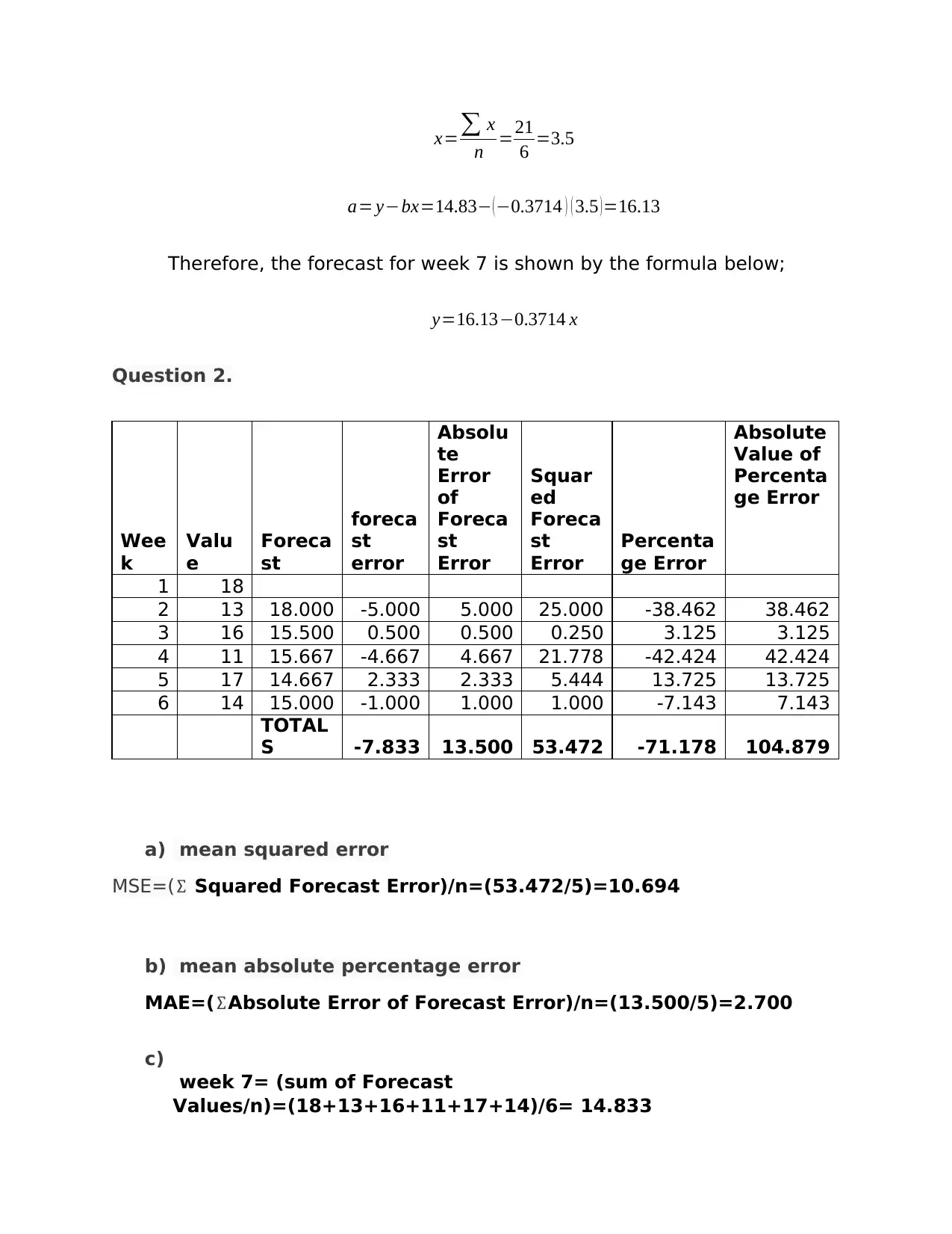
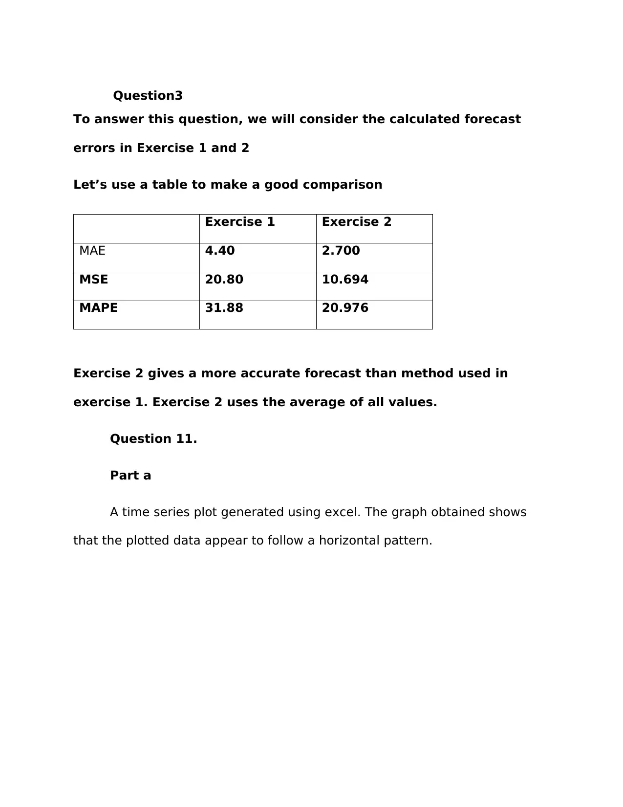
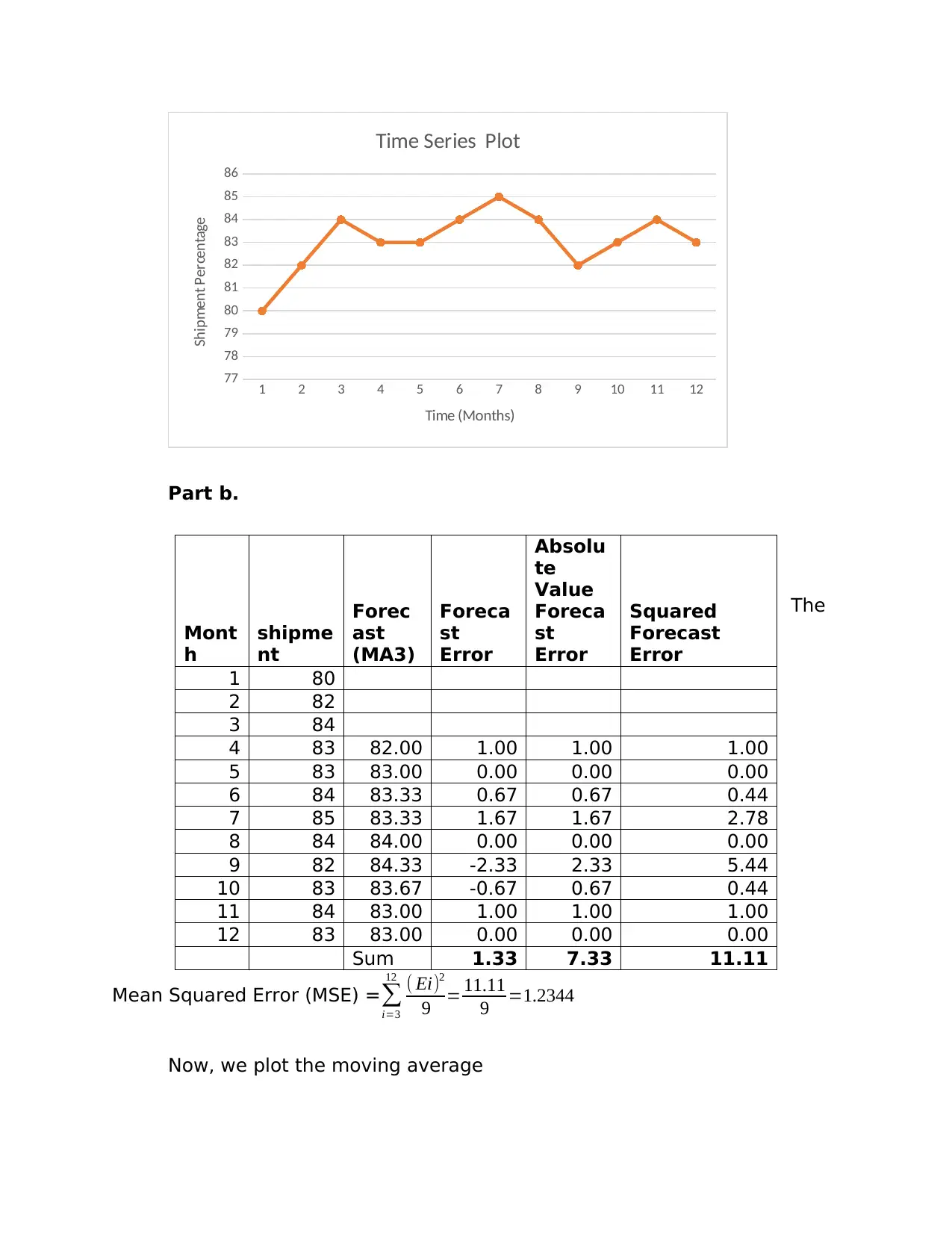
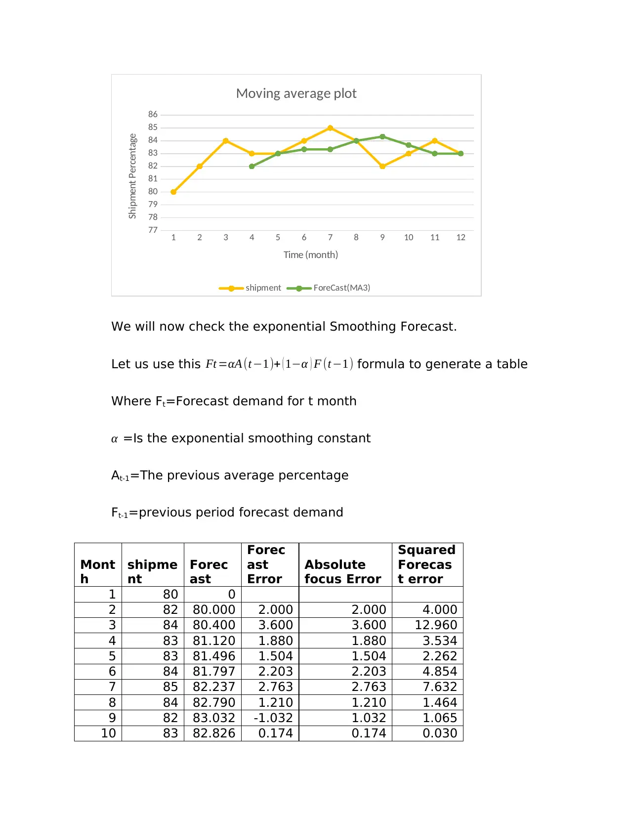
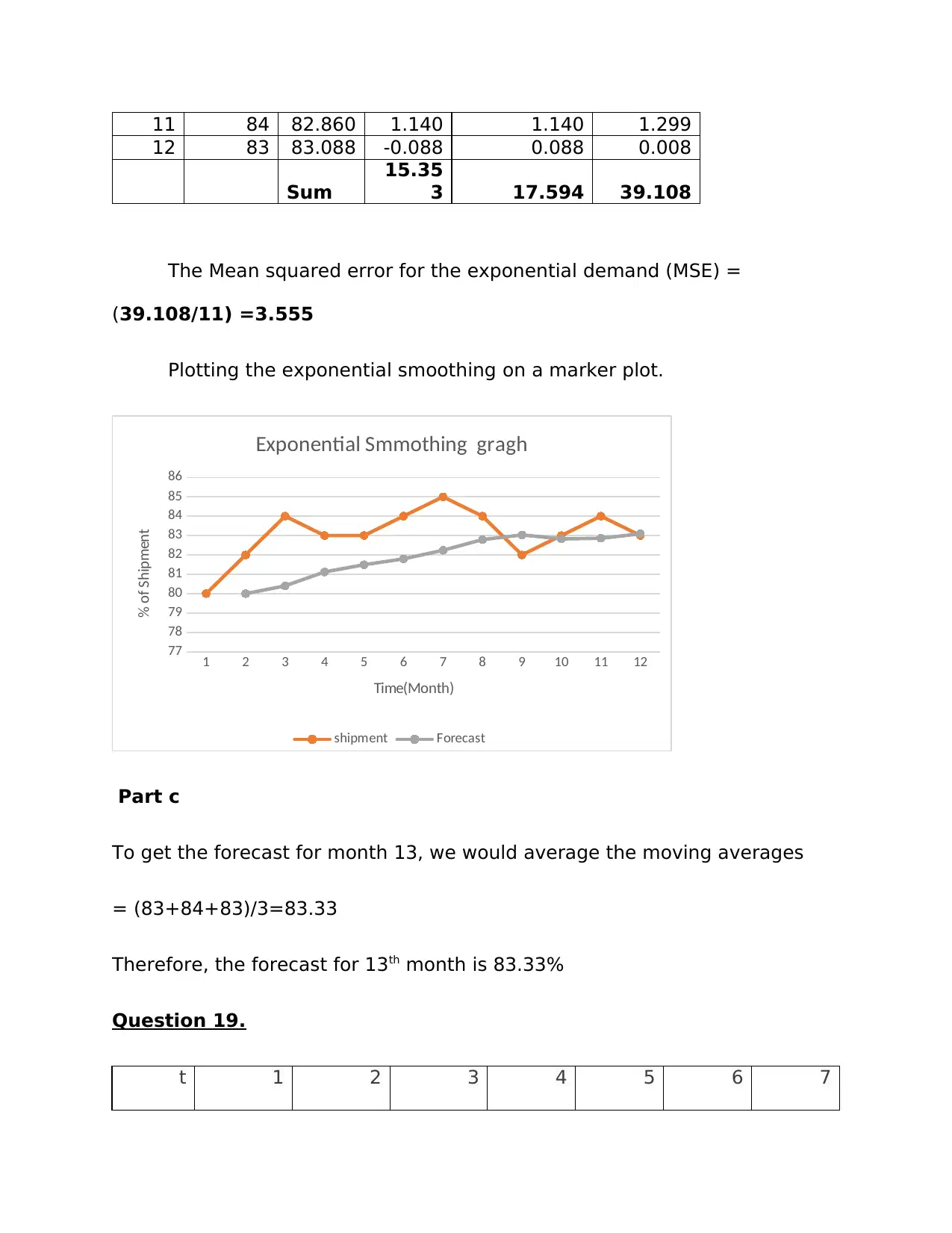
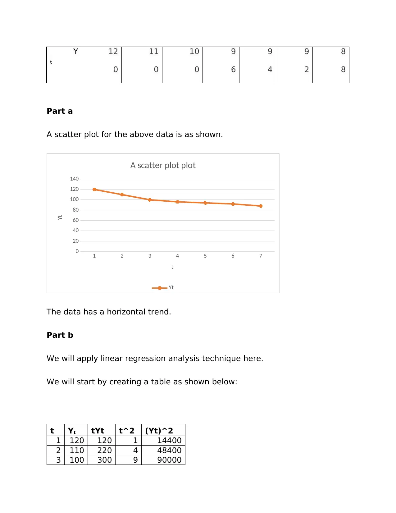
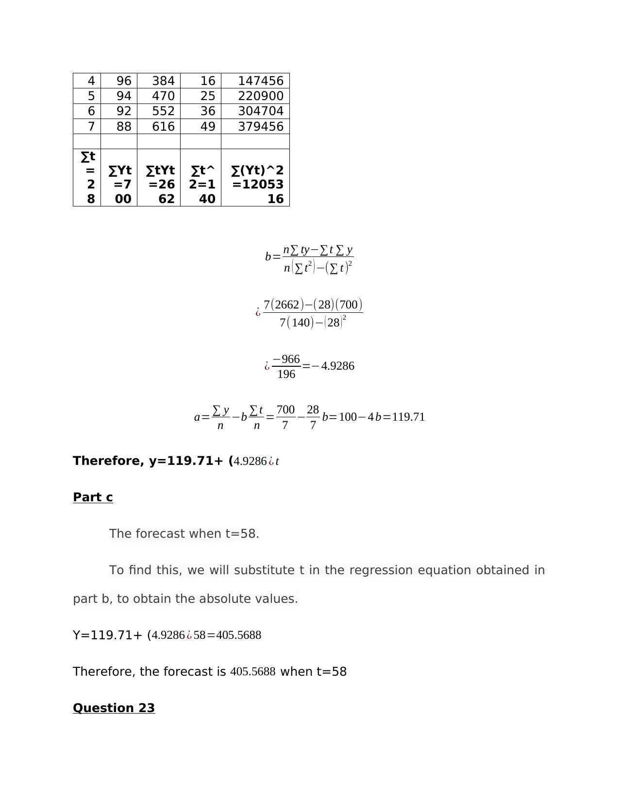
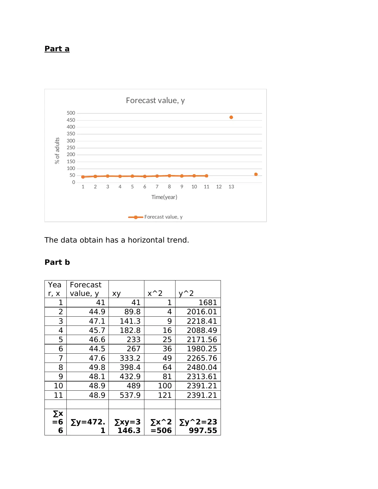
This document presents a detailed solution to a Business Decision Analysis assignment, focusing on forecasting techniques and time series analysis. The solution addresses several questions, including calculating Mean Absolute Error (MAE), Mean Squared Error (MSE), and Mean Absolute Percentage Error (MAPE) using both the naive method and the average of historical data. It also involves linear regression analysis to forecast future values and includes the creation and interpretation of time series plots, such as moving average and exponential smoothing graphs. The assignment covers questions related to forecasting shipment percentages, analyzing trends, and predicting future outcomes based on given data. The solution demonstrates the application of these statistical methods to real-world business scenarios, providing a comprehensive understanding of the concepts involved.

Kwaku Tweneboa Kodua
Yorkville University
BUSI 2013 Business Decision Analysis
Individual Problem 2
Professor: Aniket Mahanti
April 19th, 2019

Question 1
Wee
k
1 2 3 4 5 6
Valu
e
18 13 16 11 17 14
It can be solved using excel table as below.
Wee
k
Valu
e
Forecas
t Error
Forec
ast
Error
Absolut
e value
for
forecas
t error
Squar
ed
Forec
ast
Error
Percent
age
Error
Absolut
e Value
of
Percent
age
Error
1 18
2 13 18 -5 5 25 -38.4615 38.4615
3 16 13 3 3 9 18.7500 18.7500
4 11 16 -5 5 25 -45.4545 45.4545
5 17 11 6 6 36 35.2941 35.2941
6 14 17 -3 3 9 -21.4286 21.4286
Totals -4 22 104
-
51.3005
159.388
8
Alternatively, we can let the F denotes the Forecast for t period, At to denote
the actual value in t period, and Et to denote the forecast error in t period.
Now the Naïve forecast for the value in t weeks be given by
Ft=At-1

F2=A1=18
E2=A2-F1=13-18=-5
F3=A2=13
E3=A3-F2=16-13=3
F4=A3=16
E4=A4-F3=11-16=-5
F5 =A4 =11
E5 =A5-F4=17- 11=6
F6=A5 =17
E6=A6 -F5=14-17=-3
Part a
Mean Absolute Error (MAE) =∑
i=2
6 |Ei|
5 = (5+ 3+5+6+3 )
5 =4.40
Part b
Mean Squared Error (MSE) =∑
i=2
6 ( Ei)2
5 ¿
[52 +32+52+62 +32 ] /5=20.80
Part c
Mean Absolute Percentage Error (MAPE) =100 % /5 ∑
i=2
6
¿ Et
At ∨¿

¿ 100/5 ∑
i=2
6
[|−5
13 |+| 3
16 |+|−5
11 |+| 6
17|+|−3
14 |]=31.88 %
Part d
To find the forecast for week 7, we will use the formula for linear
regression stated below where b will represent the forecast for week 7.
y=a+bx
Where b= n∑ xy−∑ x ∑ y
n ¿ ¿
Wee
k (x)
Valu
e (y) xy x^2 y^2
1 18 18 1 324
2 13 26 4 169
3 16 48 9 256
4 11 44 16 121
5 17 85 25 289
6 14 84 36 196
∑x=2
1
∑y=8
9
∑xy=3
05
∑x^2
=91
∑y^2=1
355
b= 6 ( 305 )−(21)( 89)
6 ( 91 )−(21)2
b=1830− ( 1869 )
546−441 =−39
105 =−0.3714
y= ∑ y
n = 89
6 =14.83

x=∑ x
n =21
6 =3.5
a= y−bx=14.83− (−0.3714 ) ( 3.5 )=16.13
Therefore, the forecast for week 7 is shown by the formula below;
y=16.13−0.3714 x
Question 2.
Wee
k
Valu
e
Foreca
st
foreca
st
error
Absolu
te
Error
of
Foreca
st
Error
Squar
ed
Foreca
st
Error
Percenta
ge Error
Absolute
Value of
Percenta
ge Error
1 18
2 13 18.000 -5.000 5.000 25.000 -38.462 38.462
3 16 15.500 0.500 0.500 0.250 3.125 3.125
4 11 15.667 -4.667 4.667 21.778 -42.424 42.424
5 17 14.667 2.333 2.333 5.444 13.725 13.725
6 14 15.000 -1.000 1.000 1.000 -7.143 7.143
TOTAL
S -7.833 13.500 53.472 -71.178 104.879
a) mean squared error
MSE=(∑ Squared Forecast Error)/n=(53.472/5)=10.694
b) mean absolute percentage error
MAE=(∑Absolute Error of Forecast Error)/n=(13.500/5)=2.700
c)
week 7= (sum of Forecast
Values/n)=(18+13+16+11+17+14)/6= 14.833

Question3
To answer this question, we will consider the calculated forecast
errors in Exercise 1 and 2
Let’s use a table to make a good comparison
Exercise 1 Exercise 2
MAE 4.40 2.700
MSE 20.80 10.694
MAPE 31.88 20.976
Exercise 2 gives a more accurate forecast than method used in
exercise 1. Exercise 2 uses the average of all values.
Question 11.
Part a
A time series plot generated using excel. The graph obtained shows
that the plotted data appear to follow a horizontal pattern.

1 2 3 4 5 6 7 8 9 10 11 12
77
78
79
80
81
82
83
84
85
86
Time Series Plot
Time (Months)
Shipment Percentage
Part b.
The
Mean Squared Error (MSE) =∑
i=3
12 ( Ei)2
9 = 11.11
9 =1.2344
Now, we plot the moving average
Mont
h
shipme
nt
Forec
ast
(MA3)
Foreca
st
Error
Absolu
te
Value
Foreca
st
Error
Squared
Forecast
Error
1 80
2 82
3 84
4 83 82.00 1.00 1.00 1.00
5 83 83.00 0.00 0.00 0.00
6 84 83.33 0.67 0.67 0.44
7 85 83.33 1.67 1.67 2.78
8 84 84.00 0.00 0.00 0.00
9 82 84.33 -2.33 2.33 5.44
10 83 83.67 -0.67 0.67 0.44
11 84 83.00 1.00 1.00 1.00
12 83 83.00 0.00 0.00 0.00
Sum 1.33 7.33 11.11

1 2 3 4 5 6 7 8 9 10 11 12
77
78
79
80
81
82
83
84
85
86
Moving average plot
shipment ForeCast(MA3)
Time (month)
Shipment Percentage
We will now check the exponential Smoothing Forecast.
Let us use this Ft =αA (t−1)+ ( 1−α ) F (t−1) formula to generate a table
Where Ft=Forecast demand for t month
α =Is the exponential smoothing constant
At-1=The previous average percentage
Ft-1=previous period forecast demand
Mont
h
shipme
nt
Forec
ast
Forec
ast
Error
Absolute
focus Error
Squared
Forecas
t error
1 80 0
2 82 80.000 2.000 2.000 4.000
3 84 80.400 3.600 3.600 12.960
4 83 81.120 1.880 1.880 3.534
5 83 81.496 1.504 1.504 2.262
6 84 81.797 2.203 2.203 4.854
7 85 82.237 2.763 2.763 7.632
8 84 82.790 1.210 1.210 1.464
9 82 83.032 -1.032 1.032 1.065
10 83 82.826 0.174 0.174 0.030

11 84 82.860 1.140 1.140 1.299
12 83 83.088 -0.088 0.088 0.008
Sum
15.35
3 17.594 39.108
The Mean squared error for the exponential demand (MSE) =
(39.108/11) =3.555
Plotting the exponential smoothing on a marker plot.
1 2 3 4 5 6 7 8 9 10 11 12
77
78
79
80
81
82
83
84
85
86
Exponential Smmothing gragh
shipment Forecast
Time(Month)
% of Shipment
Part c
To get the forecast for month 13, we would average the moving averages
= (83+84+83)/3=83.33
Therefore, the forecast for 13th month is 83.33%
Question 19.
t 1 2 3 4 5 6 7

Y
t
12
0
11
0
10
0
9
6
9
4
9
2
8
8
Part a
A scatter plot for the above data is as shown.
1 2 3 4 5 6 7
0
20
40
60
80
100
120
140
A scatter plot plot
Yt
t
Yt
The data has a horizontal trend.
Part b
We will apply linear regression analysis technique here.
We will start by creating a table as shown below:
t Yt tYt t^2 (Yt)^2
1 120 120 1 14400
2 110 220 4 48400
3 100 300 9 90000

4 96 384 16 147456
5 94 470 25 220900
6 92 552 36 304704
7 88 616 49 379456
∑t
=
2
8
∑Yt
=7
00
∑tYt
=26
62
∑t^
2=1
40
∑(Yt)^2
=12053
16
b= n∑ ty−∑t ∑ y
n ( ∑ t2 ) −(∑ t)2
¿ 7(2662)−( 28)(700)
7(140)− ( 28 )2
¿ −966
196 =−4.9286
a= ∑ y
n −b ∑ t
n = 700
7 −28
7 b=100−4 b=119.71
Therefore, y=119.71+ ( 4.9286 ¿ t
Part c
The forecast when t=58.
To find this, we will substitute t in the regression equation obtained in
part b, to obtain the absolute values.
Y=119.71+ ( 4.9286 ¿ 58=405.5688
Therefore, the forecast is 405.5688 when t=58
Question 23

Part a
1 2 3 4 5 6 7 8 9 10 11 12 13
0
50
100
150
200
250
300
350
400
450
500
Forecast value, y
Forecast value, y
Time(year)
% of adults
The data obtain has a horizontal trend.
Part b
Yea
r, x
Forecast
value, y xy x^2 y^2
1 41 41 1 1681
2 44.9 89.8 4 2016.01
3 47.1 141.3 9 2218.41
4 45.7 182.8 16 2088.49
5 46.6 233 25 2171.56
6 44.5 267 36 1980.25
7 47.6 333.2 49 2265.76
8 49.8 398.4 64 2480.04
9 48.1 432.9 81 2313.61
10 48.9 489 100 2391.21
11 48.9 537.9 121 2391.21
∑x
=6
6
∑y=472.
1
∑xy=3
146.3
∑x^2
=506
∑y^2=23
997.55