Business Analysis and Statistical Report: Harvest Kitchen Performance
VerifiedAdded on 2020/04/07
|17
|3550
|222
Report
AI Summary
This report analyzes the business performance of a small health food shop, Harvest Kitchen, on the Sunshine Coast, focusing on sales, profit, and payment methods. The analysis includes descriptive statistics, box plots, and inferential statistics like paired t-tests and ANOVA to evaluate sales across different payment methods, product locations, and seasons. Key findings reveal that credit card payments yield the highest returns, and the outside front product position generates the most profit. While seasonal sales are not significantly different, profit varies, with spring being the most profitable. The report also examines the relationship between rainfall and profit and determines that the average net sale is not significantly different in all the months of the year. The analysis provides valuable insights for business management, including recommendations for optimizing payment methods, product placement, and seasonal strategies.

Surname 1
Business analysis and statistics
Name
The Name of the Class (Course)
Professor (Tutor)
The Name of the School (University)
The City and State where it is located
Date
Business analysis and statistics
Name
The Name of the Class (Course)
Professor (Tutor)
The Name of the School (University)
The City and State where it is located
Date
Paraphrase This Document
Need a fresh take? Get an instant paraphrase of this document with our AI Paraphraser
Surname 2
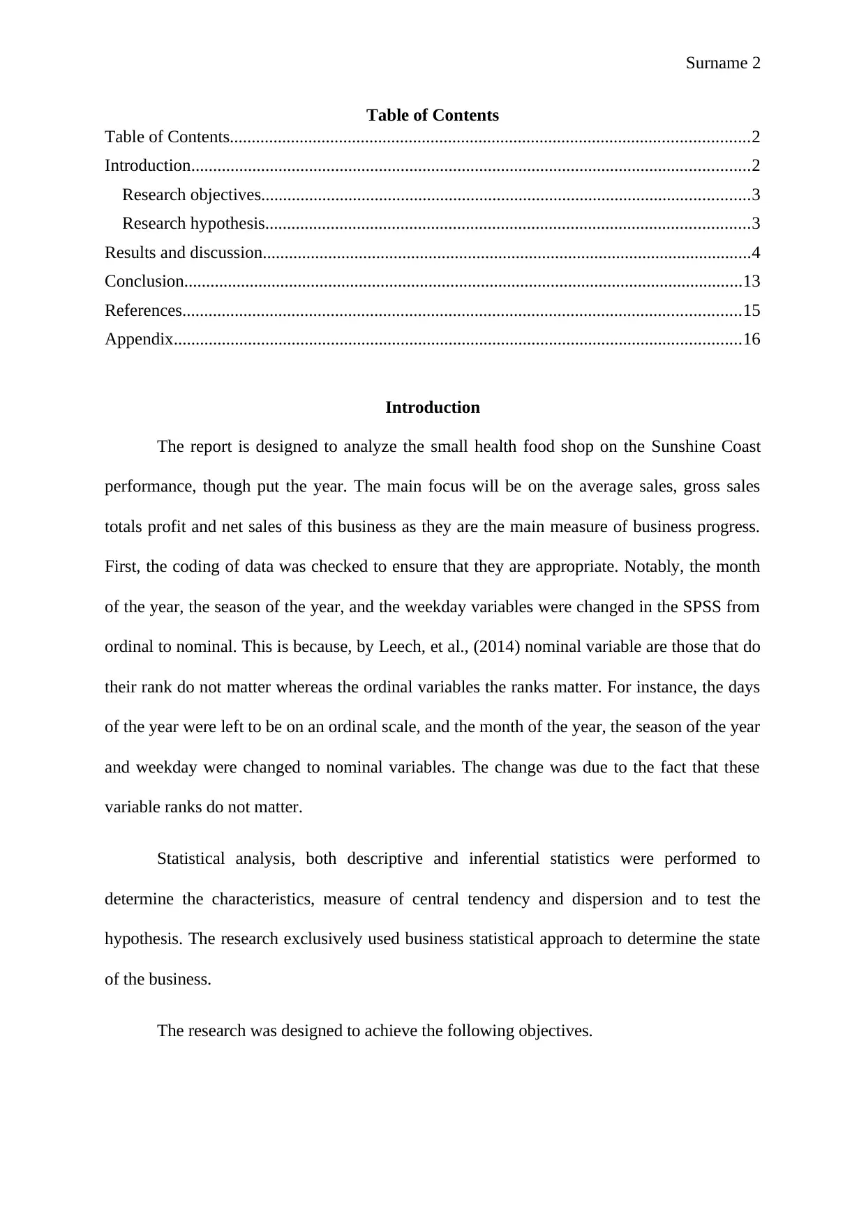
Table of Contents
Table of Contents.......................................................................................................................2
Introduction................................................................................................................................2
Research objectives................................................................................................................3
Research hypothesis...............................................................................................................3
Results and discussion................................................................................................................4
Conclusion................................................................................................................................13
References................................................................................................................................15
Appendix..................................................................................................................................16
Introduction
The report is designed to analyze the small health food shop on the Sunshine Coast
performance, though put the year. The main focus will be on the average sales, gross sales
totals profit and net sales of this business as they are the main measure of business progress.
First, the coding of data was checked to ensure that they are appropriate. Notably, the month
of the year, the season of the year, and the weekday variables were changed in the SPSS from
ordinal to nominal. This is because, by Leech, et al., (2014) nominal variable are those that do
their rank do not matter whereas the ordinal variables the ranks matter. For instance, the days
of the year were left to be on an ordinal scale, and the month of the year, the season of the year
and weekday were changed to nominal variables. The change was due to the fact that these
variable ranks do not matter.
Statistical analysis, both descriptive and inferential statistics were performed to
determine the characteristics, measure of central tendency and dispersion and to test the
hypothesis. The research exclusively used business statistical approach to determine the state
of the business.
The research was designed to achieve the following objectives.
Surname 3
Research objectives
The report was designed to achieve the following objectives;
Describe the distribution of the variables that evaluate the performance of the
small health food shop on the Sunshine Coast.
Determine whether the sales are equal in all the seasons.
Determine whether the profit differs from season to season.
Determine whether the profit differs in different months.
Give recommendation based on the findings.
Research hypothesis
The analysis focused on testing the hypotheses:
1. H0: the average performance of different methods of payment is equal.
H1: the average performance of different methods of payment is equal.
2. H0: there is no difference in the average sale of different product location
H1: there is a significant sales average difference by the product location.
3. H0: the average net profit accrued from different selling position is not significantly
different
H1: the average net profit accrued from different selling position is significantly
different.
4. H0: The net sales in different seasons of the year were not different.
H1: The net sales in different seasons of the year were different.
The analysis was designed to give a detailed discussion of the findings, obtained when
assessing the given hypothesis.
⊘ This is a preview!⊘
Do you want full access?
Subscribe today to unlock all pages.
Trusted by 1+ million students worldwide
Surname 4
Results and discussion
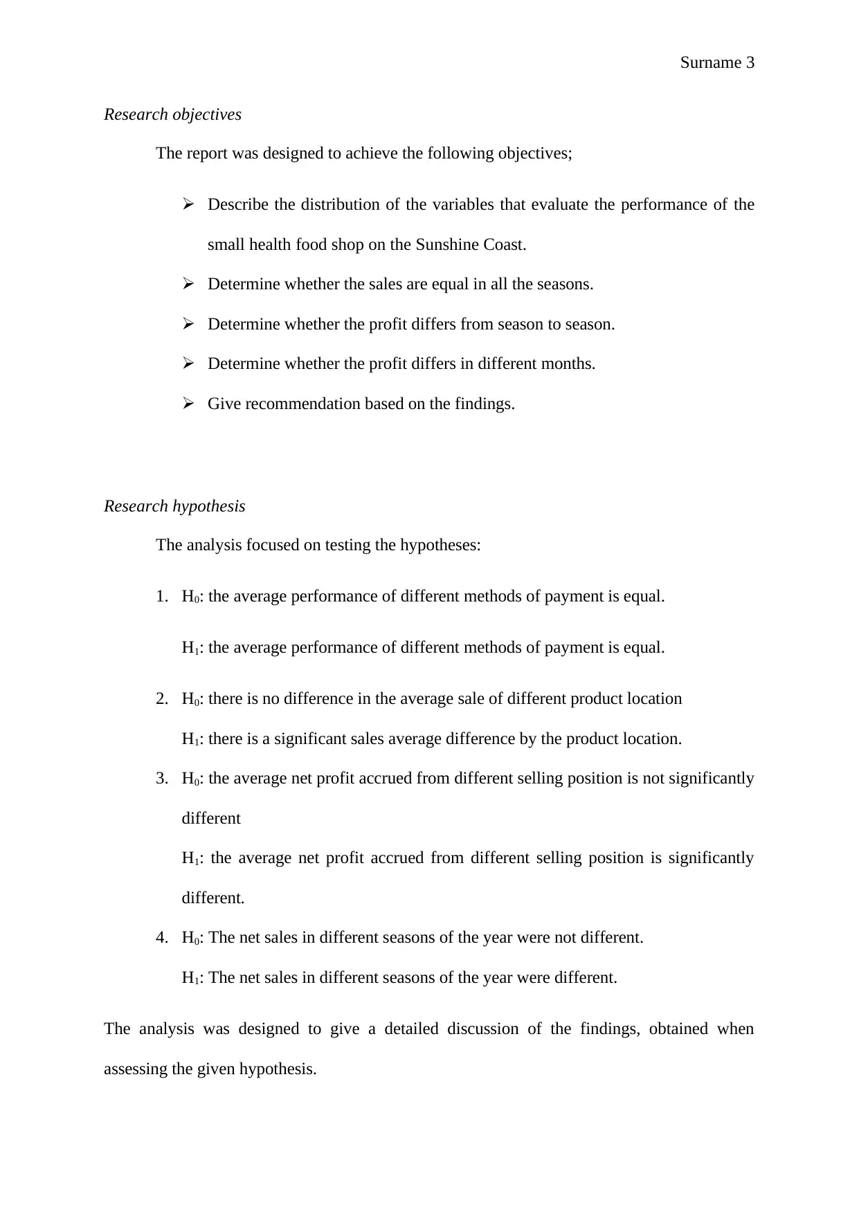
Descriptive statistics for the net sales, average sales, profit total and cash total, were
computed. The results are as summarized in Table 1.
Table 1: Descriptive statistics
Descriptive Statistics
N Range Minimum Maximum Mean Std. Deviation Skewness
Statistic Statistic Statistic Statistic Statistic Statistic Statistic Std. Error
Net_Sales 366 2370 0 2370 1014.26 313.986 -.362 .128
Average_Sale 358 53 8 61 18.52 3.985 3.758 .129
Profit Total 366 305.95 -33.98 271.97 30.7098 30.05661 3.274 .128
Cash_Total 366 1195 0 1195 404.29 153.643 .490 .128
Valid N (listwise) 358
The average net sale is $1,014.26 (SD = $313.99). The minimum net sale zero and the
maximum of $2,370, meaning that the range is $2,370. The net sale has a negatively skewed
plot, but it is not that much skewed. The average sales mean is $18.52 (SD = $3.99). The
skewness coefficient shows that the average sales data are very skewed since the coefficient is
greater than 2.00 (Kim, 2013). The same distribution is seen in the profit total, which has an
average of $30.06 (SD = $3.27). Lastly, the cash total average is $404.29 (SD = $153.64). The
data distribution is not that skewed since it is close to zero (Blanca, et al., 2013).
Results and discussion
Descriptive statistics for the net sales, average sales, profit total and cash total, were
computed. The results are as summarized in Table 1.
Table 1: Descriptive statistics
Descriptive Statistics
N Range Minimum Maximum Mean Std. Deviation Skewness
Statistic Statistic Statistic Statistic Statistic Statistic Statistic Std. Error
Net_Sales 366 2370 0 2370 1014.26 313.986 -.362 .128
Average_Sale 358 53 8 61 18.52 3.985 3.758 .129
Profit Total 366 305.95 -33.98 271.97 30.7098 30.05661 3.274 .128
Cash_Total 366 1195 0 1195 404.29 153.643 .490 .128
Valid N (listwise) 358
The average net sale is $1,014.26 (SD = $313.99). The minimum net sale zero and the
maximum of $2,370, meaning that the range is $2,370. The net sale has a negatively skewed
plot, but it is not that much skewed. The average sales mean is $18.52 (SD = $3.99). The
skewness coefficient shows that the average sales data are very skewed since the coefficient is
greater than 2.00 (Kim, 2013). The same distribution is seen in the profit total, which has an
average of $30.06 (SD = $3.27). Lastly, the cash total average is $404.29 (SD = $153.64). The
data distribution is not that skewed since it is close to zero (Blanca, et al., 2013).
Paraphrase This Document
Need a fresh take? Get an instant paraphrase of this document with our AI Paraphraser
Surname 5
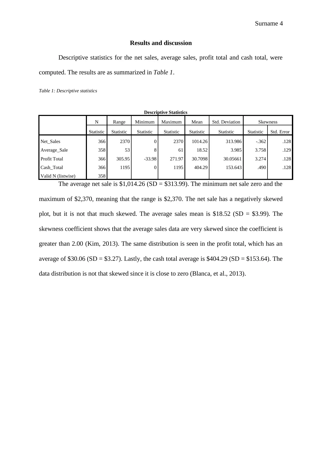
Figure 1: Boxplot of Gross sale
Figure 1 shows that the data are relative normally distributed around the measure of central
tendency. However, there are a few outliers on both side of the tails.
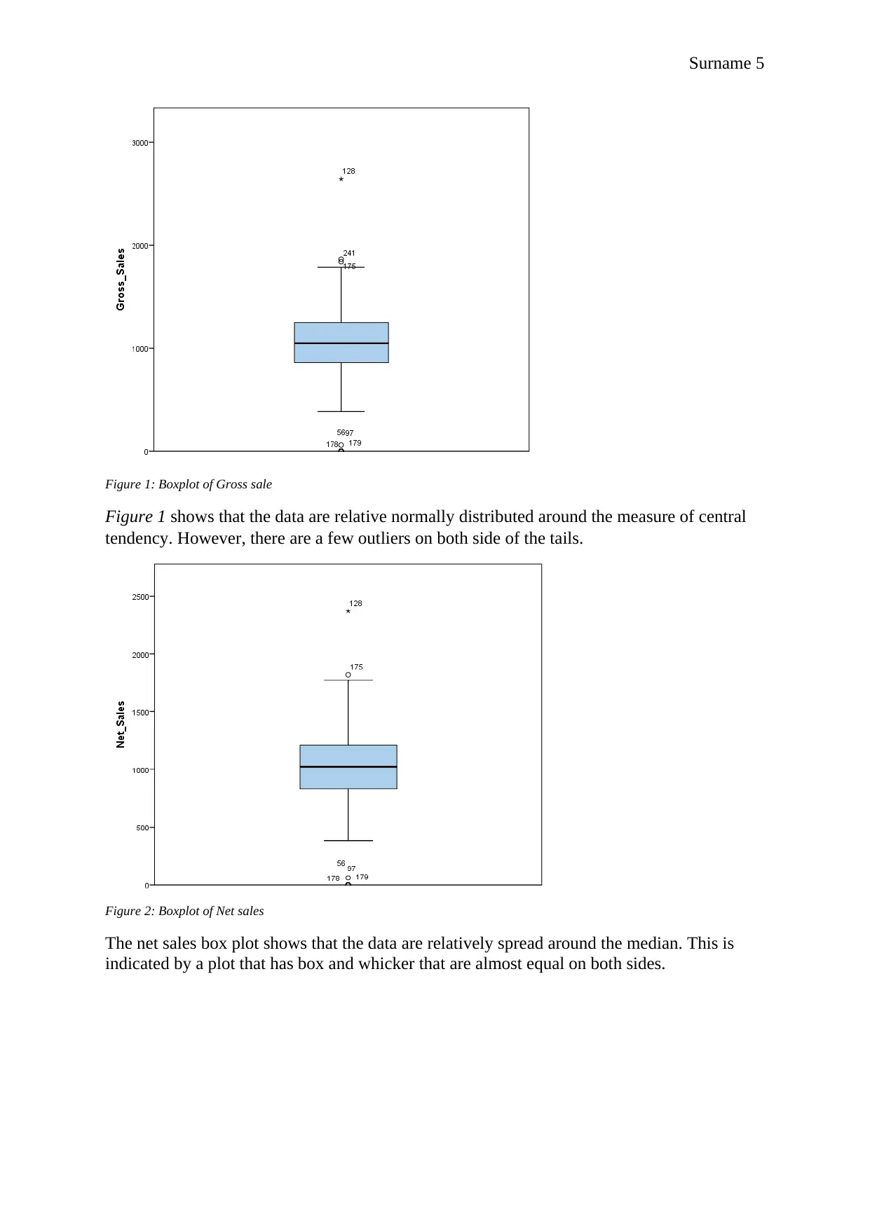
Figure 2: Boxplot of Net sales
The net sales box plot shows that the data are relatively spread around the median. This is
indicated by a plot that has box and whicker that are almost equal on both sides.
Figure 1: Boxplot of Gross sale
Figure 1 shows that the data are relative normally distributed around the measure of central
tendency. However, there are a few outliers on both side of the tails.
Figure 2: Boxplot of Net sales
The net sales box plot shows that the data are relatively spread around the median. This is
indicated by a plot that has box and whicker that are almost equal on both sides.
Surname 6
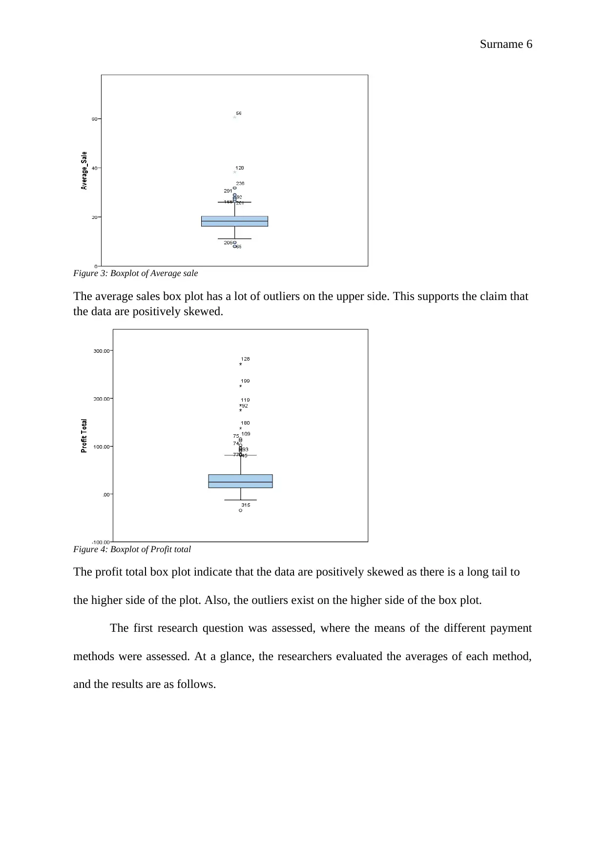
Figure 3: Boxplot of Average sale
The average sales box plot has a lot of outliers on the upper side. This supports the claim that
the data are positively skewed.
Figure 4: Boxplot of Profit total
The profit total box plot indicate that the data are positively skewed as there is a long tail to
the higher side of the plot. Also, the outliers exist on the higher side of the box plot.
The first research question was assessed, where the means of the different payment
methods were assessed. At a glance, the researchers evaluated the averages of each method,
and the results are as follows.
⊘ This is a preview!⊘
Do you want full access?
Subscribe today to unlock all pages.
Trusted by 1+ million students worldwide
Surname 7
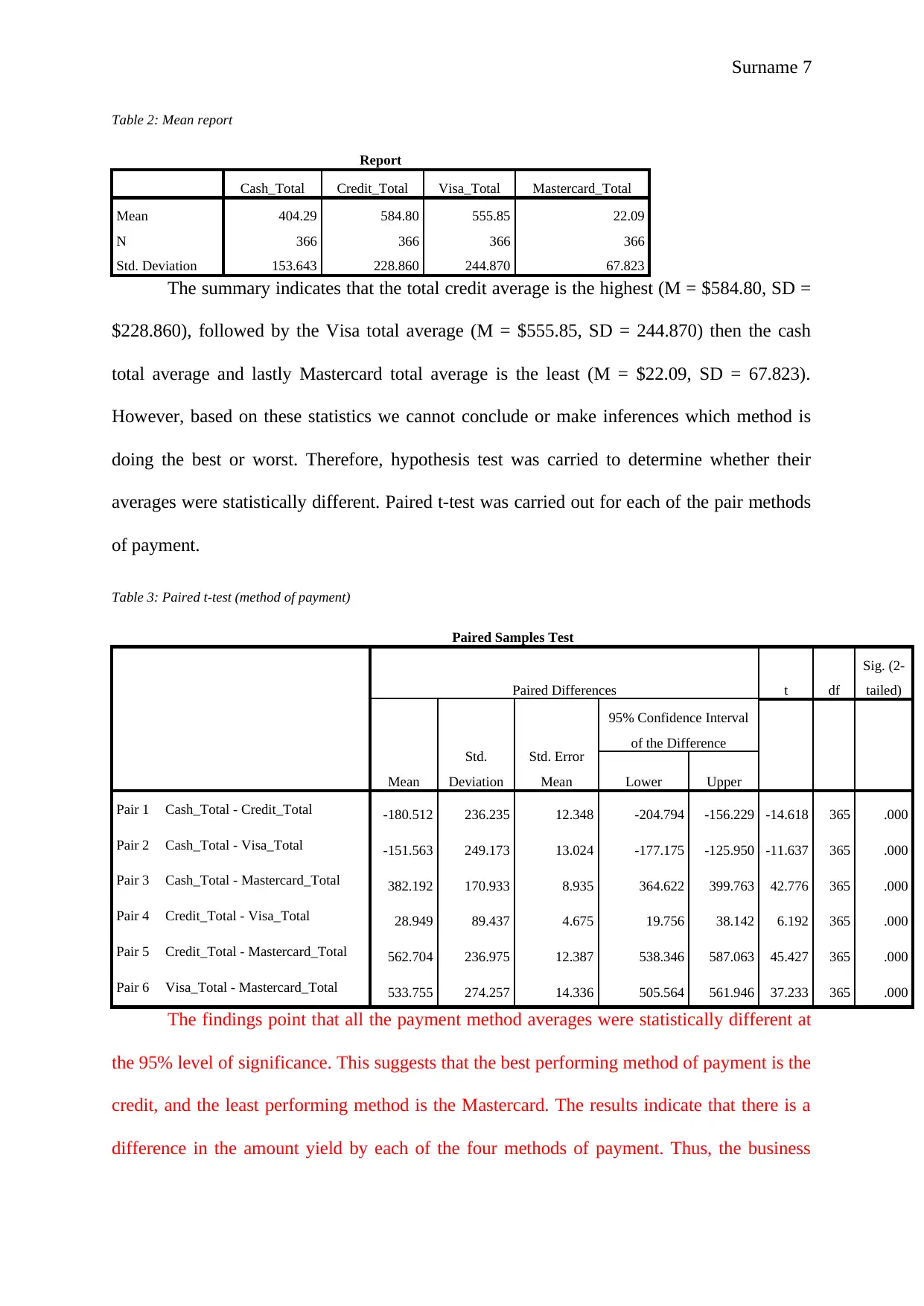
Table 2: Mean report
Report
Cash_Total Credit_Total Visa_Total Mastercard_Total
Mean 404.29 584.80 555.85 22.09
N 366 366 366 366
Std. Deviation 153.643 228.860 244.870 67.823
The summary indicates that the total credit average is the highest (M = $584.80, SD =
$228.860), followed by the Visa total average (M = $555.85, SD = 244.870) then the cash
total average and lastly Mastercard total average is the least (M = $22.09, SD = 67.823).
However, based on these statistics we cannot conclude or make inferences which method is
doing the best or worst. Therefore, hypothesis test was carried to determine whether their
averages were statistically different. Paired t-test was carried out for each of the pair methods
of payment.
Table 3: Paired t-test (method of payment)
Paired Samples Test
Paired Differences t df
Sig. (2-
tailed)
Mean
Std.
Deviation
Std. Error
Mean
95% Confidence Interval
of the Difference
Lower Upper
Pair 1 Cash_Total - Credit_Total -180.512 236.235 12.348 -204.794 -156.229 -14.618 365 .000
Pair 2 Cash_Total - Visa_Total -151.563 249.173 13.024 -177.175 -125.950 -11.637 365 .000
Pair 3 Cash_Total - Mastercard_Total 382.192 170.933 8.935 364.622 399.763 42.776 365 .000
Pair 4 Credit_Total - Visa_Total 28.949 89.437 4.675 19.756 38.142 6.192 365 .000
Pair 5 Credit_Total - Mastercard_Total 562.704 236.975 12.387 538.346 587.063 45.427 365 .000
Pair 6 Visa_Total - Mastercard_Total 533.755 274.257 14.336 505.564 561.946 37.233 365 .000
The findings point that all the payment method averages were statistically different at
the 95% level of significance. This suggests that the best performing method of payment is the
credit, and the least performing method is the Mastercard. The results indicate that there is a
difference in the amount yield by each of the four methods of payment. Thus, the business
Paraphrase This Document
Need a fresh take? Get an instant paraphrase of this document with our AI Paraphraser
Surname 8
should emphasize the use of the most common mode of payment which is credit followed by
the visa. The Mastercard seems to be doing very poorly, which can mean that it is not well
recognized in this area.
Second, the research question was answered through testing the hypothesis: H0: there
is no difference in the average sale of different product location, Vs. H1: there is a significant
sales average difference by the product location. One-way ANOVA was carried out, and the
findings are summarized in
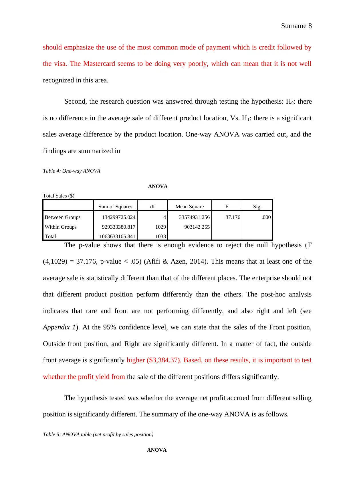
Table 4: One-way ANOVA
ANOVA
Total Sales ($)
Sum of Squares df Mean Square F Sig.
Between Groups 134299725.024 4 33574931.256 37.176 .000
Within Groups 929333380.817 1029 903142.255
Total 1063633105.841 1033
The p-value shows that there is enough evidence to reject the null hypothesis (F
(4,1029) = 37.176, p-value < .05) (Afifi & Azen, 2014). This means that at least one of the
average sale is statistically different than that of the different places. The enterprise should not
that different product position perform differently than the others. The post-hoc analysis
indicates that rare and front are not performing differently, and also right and left (see
Appendix 1). At the 95% confidence level, we can state that the sales of the Front position,
Outside front position, and Right are significantly different. In a matter of fact, the outside
front average is significantly higher ($3,384.37). Based, on these results, it is important to test
whether the profit yield from the sale of the different positions differs significantly.
The hypothesis tested was whether the average net profit accrued from different selling
position is significantly different. The summary of the one-way ANOVA is as follows.
Table 5: ANOVA table (net profit by sales position)
ANOVA
should emphasize the use of the most common mode of payment which is credit followed by
the visa. The Mastercard seems to be doing very poorly, which can mean that it is not well
recognized in this area.
Second, the research question was answered through testing the hypothesis: H0: there
is no difference in the average sale of different product location, Vs. H1: there is a significant
sales average difference by the product location. One-way ANOVA was carried out, and the
findings are summarized in
Table 4: One-way ANOVA
ANOVA
Total Sales ($)
Sum of Squares df Mean Square F Sig.
Between Groups 134299725.024 4 33574931.256 37.176 .000
Within Groups 929333380.817 1029 903142.255
Total 1063633105.841 1033
The p-value shows that there is enough evidence to reject the null hypothesis (F
(4,1029) = 37.176, p-value < .05) (Afifi & Azen, 2014). This means that at least one of the
average sale is statistically different than that of the different places. The enterprise should not
that different product position perform differently than the others. The post-hoc analysis
indicates that rare and front are not performing differently, and also right and left (see
Appendix 1). At the 95% confidence level, we can state that the sales of the Front position,
Outside front position, and Right are significantly different. In a matter of fact, the outside
front average is significantly higher ($3,384.37). Based, on these results, it is important to test
whether the profit yield from the sale of the different positions differs significantly.
The hypothesis tested was whether the average net profit accrued from different selling
position is significantly different. The summary of the one-way ANOVA is as follows.
Table 5: ANOVA table (net profit by sales position)
ANOVA
Surname 9
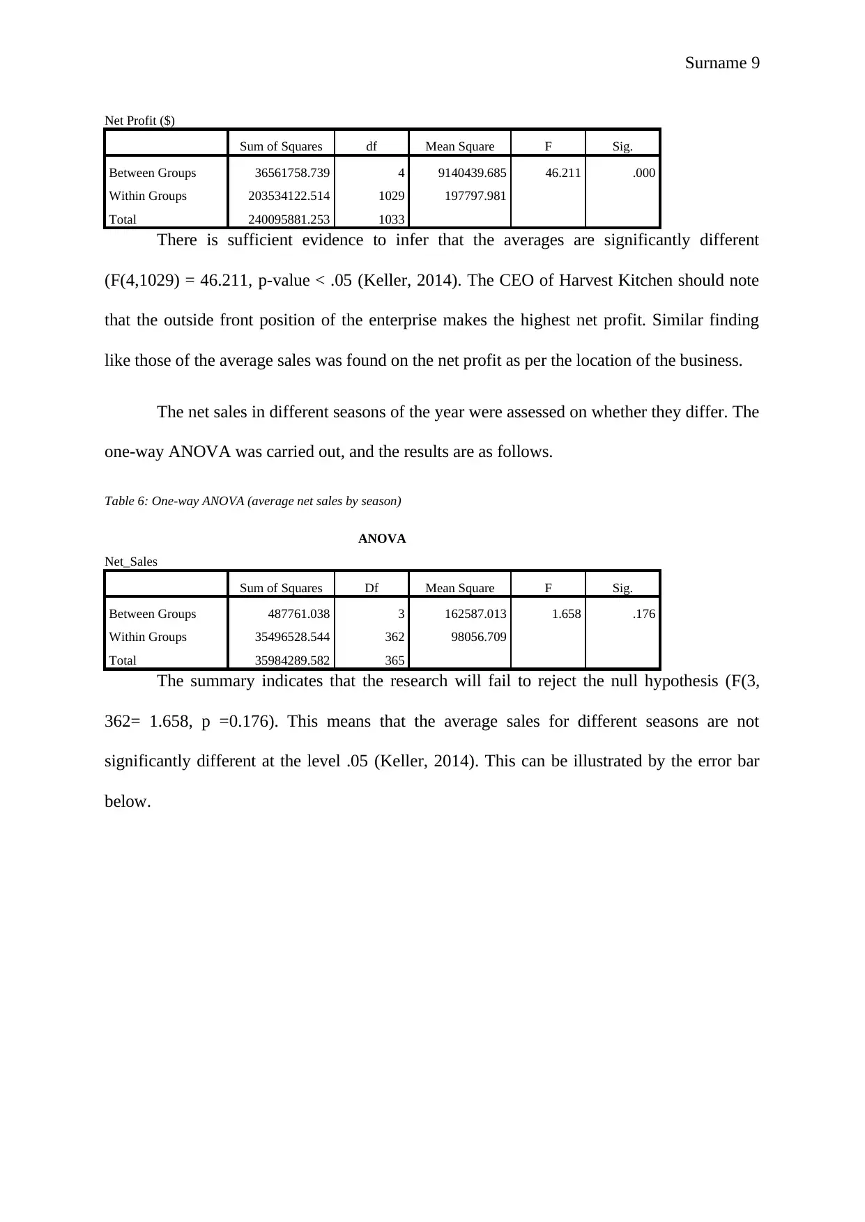
Net Profit ($)
Sum of Squares df Mean Square F Sig.
Between Groups 36561758.739 4 9140439.685 46.211 .000
Within Groups 203534122.514 1029 197797.981
Total 240095881.253 1033
There is sufficient evidence to infer that the averages are significantly different
(F(4,1029) = 46.211, p-value < .05 (Keller, 2014). The CEO of Harvest Kitchen should note
that the outside front position of the enterprise makes the highest net profit. Similar finding
like those of the average sales was found on the net profit as per the location of the business.
The net sales in different seasons of the year were assessed on whether they differ. The
one-way ANOVA was carried out, and the results are as follows.
Table 6: One-way ANOVA (average net sales by season)
ANOVA
Net_Sales
Sum of Squares Df Mean Square F Sig.
Between Groups 487761.038 3 162587.013 1.658 .176
Within Groups 35496528.544 362 98056.709
Total 35984289.582 365
The summary indicates that the research will fail to reject the null hypothesis (F(3,
362= 1.658, p =0.176). This means that the average sales for different seasons are not
significantly different at the level .05 (Keller, 2014). This can be illustrated by the error bar
below.
⊘ This is a preview!⊘
Do you want full access?
Subscribe today to unlock all pages.
Trusted by 1+ million students worldwide
Surname 10
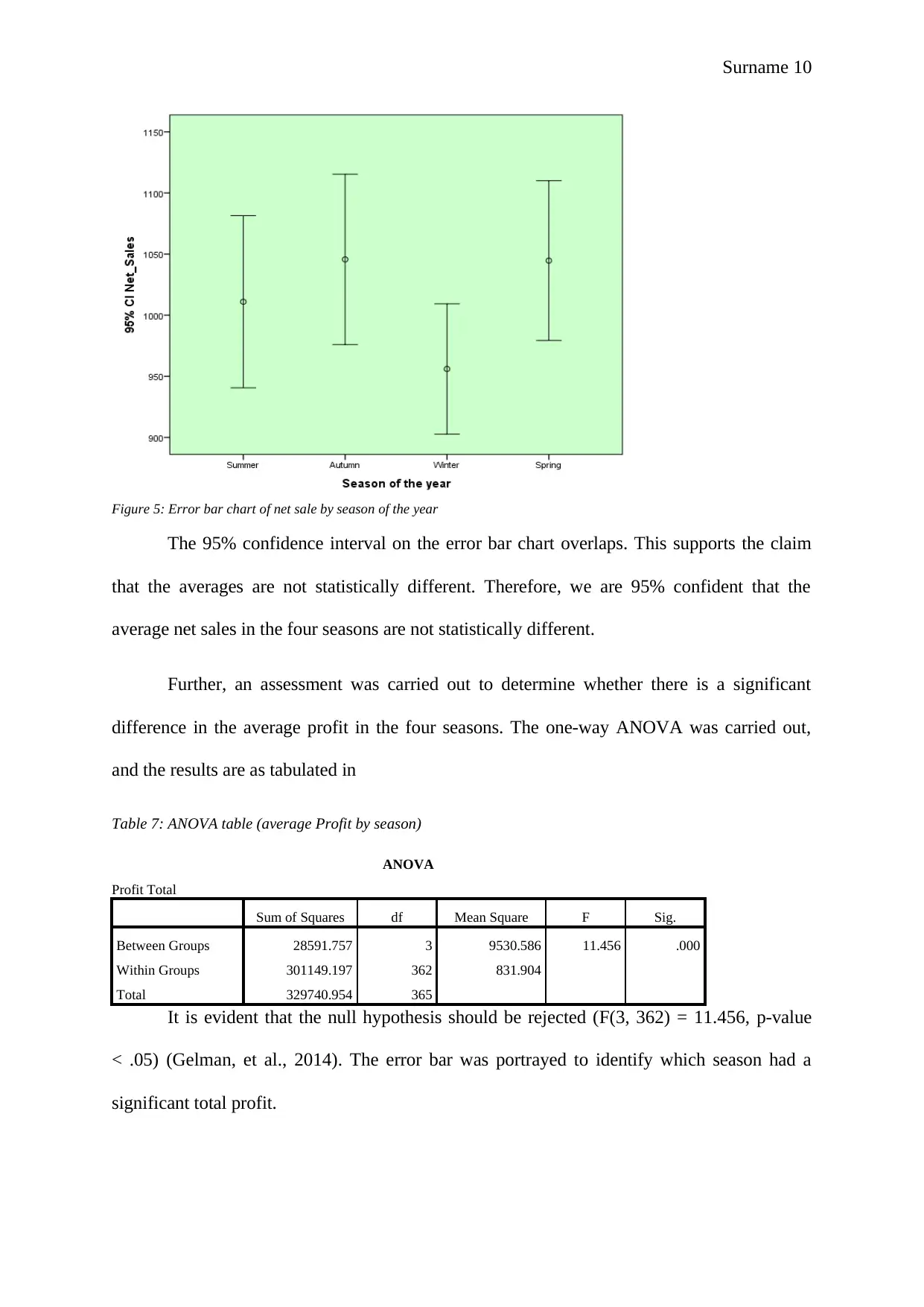
Figure 5: Error bar chart of net sale by season of the year
The 95% confidence interval on the error bar chart overlaps. This supports the claim
that the averages are not statistically different. Therefore, we are 95% confident that the
average net sales in the four seasons are not statistically different.
Further, an assessment was carried out to determine whether there is a significant
difference in the average profit in the four seasons. The one-way ANOVA was carried out,
and the results are as tabulated in
Table 7: ANOVA table (average Profit by season)
ANOVA
Profit Total
Sum of Squares df Mean Square F Sig.
Between Groups 28591.757 3 9530.586 11.456 .000
Within Groups 301149.197 362 831.904
Total 329740.954 365
It is evident that the null hypothesis should be rejected (F(3, 362) = 11.456, p-value
< .05) (Gelman, et al., 2014). The error bar was portrayed to identify which season had a
significant total profit.
Paraphrase This Document
Need a fresh take? Get an instant paraphrase of this document with our AI Paraphraser
Surname 11
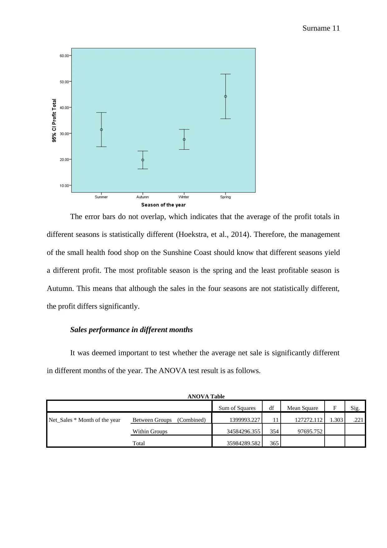
The error bars do not overlap, which indicates that the average of the profit totals in
different seasons is statistically different (Hoekstra, et al., 2014). Therefore, the management
of the small health food shop on the Sunshine Coast should know that different seasons yield
a different profit. The most profitable season is the spring and the least profitable season is
Autumn. This means that although the sales in the four seasons are not statistically different,
the profit differs significantly.
Sales performance in different months
It was deemed important to test whether the average net sale is significantly different
in different months of the year. The ANOVA test result is as follows.
ANOVA Table
Sum of Squares df Mean Square F Sig.
Net_Sales * Month of the year Between Groups (Combined) 1399993.227 11 127272.112 1.303 .221
Within Groups 34584296.355 354 97695.752
Total 35984289.582 365
Surname 12
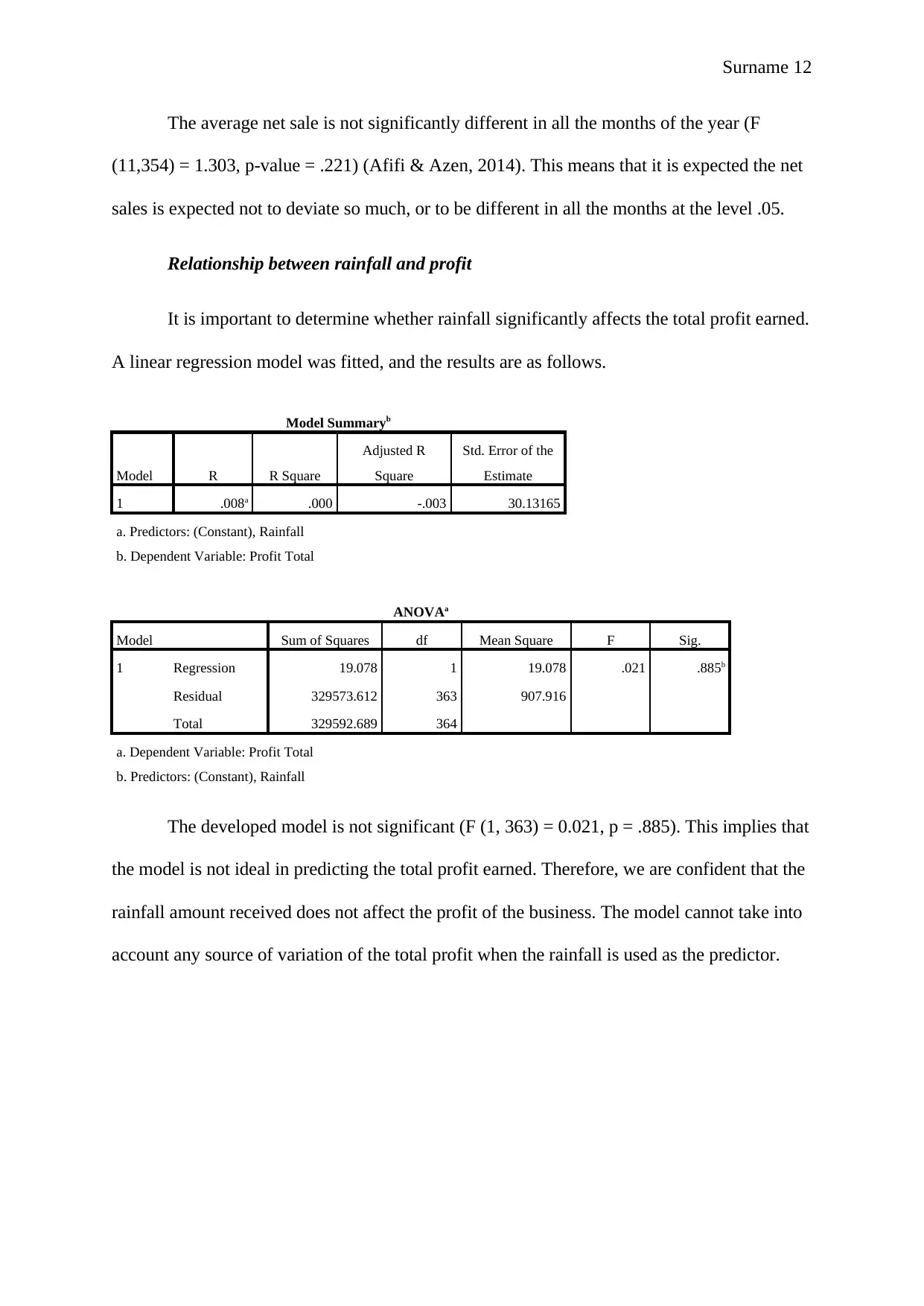
The average net sale is not significantly different in all the months of the year (F
(11,354) = 1.303, p-value = .221) (Afifi & Azen, 2014). This means that it is expected the net
sales is expected not to deviate so much, or to be different in all the months at the level .05.
Relationship between rainfall and profit
It is important to determine whether rainfall significantly affects the total profit earned.
A linear regression model was fitted, and the results are as follows.
Model Summaryb
Model R R Square
Adjusted R
Square
Std. Error of the
Estimate
1 .008a .000 -.003 30.13165
a. Predictors: (Constant), Rainfall
b. Dependent Variable: Profit Total
ANOVAa
Model Sum of Squares df Mean Square F Sig.
1 Regression 19.078 1 19.078 .021 .885b
Residual 329573.612 363 907.916
Total 329592.689 364
a. Dependent Variable: Profit Total
b. Predictors: (Constant), Rainfall
The developed model is not significant (F (1, 363) = 0.021, p = .885). This implies that
the model is not ideal in predicting the total profit earned. Therefore, we are confident that the
rainfall amount received does not affect the profit of the business. The model cannot take into
account any source of variation of the total profit when the rainfall is used as the predictor.
⊘ This is a preview!⊘
Do you want full access?
Subscribe today to unlock all pages.
Trusted by 1+ million students worldwide
1 out of 17
Related Documents


![Harvest Kitchen: Sales Performance Analysis Report - [Course Name]](/_next/image/?url=https%3A%2F%2Fdesklib.com%2Fmedia%2Fimages%2Fqi%2F14aa28e27baa43b8a0e4a08921cb48ba.jpg&w=256&q=75)


Your All-in-One AI-Powered Toolkit for Academic Success.
+13062052269
info@desklib.com
Available 24*7 on WhatsApp / Email
![[object Object]](/_next/static/media/star-bottom.7253800d.svg)
Unlock your academic potential
Copyright © 2020–2026 A2Z Services. All Rights Reserved. Developed and managed by ZUCOL.