INFS 4018 Business Analytics: House Price Prediction with Data Mining

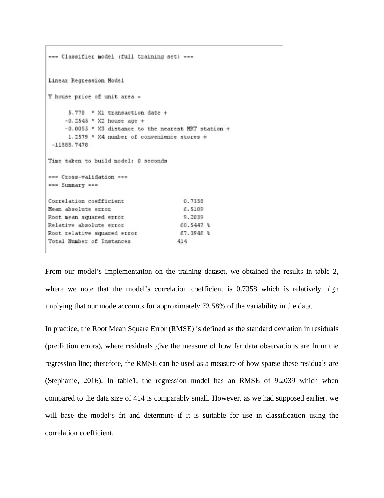
This report analyzes the factors influencing house prices in the real estate industry using data mining classification techniques, specifically multiple linear regression. The analysis explores the impact of transaction date, house age, distance to the nearest MRT station, and the number of convenience stores on house prices per unit area. The model achieves a correlation coefficient of 0.7358, indicating a relatively high accuracy in predicting house prices. Key findings suggest that transaction date and the number of convenience stores positively influence house prices, while house age and distance to the nearest MRT station have a negative impact. The report concludes with advisory actions for real estate investment, emphasizing the importance of proximity to convenience stores and the age of the house. The firm should consider investing in houses closer to convenience stores and newer houses in the short term, and building its own houses near MRT stations and convenience stores in the long term to maximize profits.

Background
With the ever growing Australian population which is projected to reach up to approximately 30
million persons in 2029, it is not surprising that several research articles report an increase in
congestion of cities, transport amenities, etcetera if the rate of developing such social amenities
does not adopt to the growing population (CBRE, 2019). However, changes in population come
as both a blessing or at times as a curse depending on the perspective of the viewer. For instance,
considering the real estate industry, increase in population translates to widening marketing
opportunities if the investors know when and how to invest.
Aim
In this paper, we will adopt the use of classification techniques to conduct an analysis of the
factors that influence the prices of houses in the real estate industry.
Methodology
Data mining method
In business and organizational practices, it is often important to put in place ways with
which to handle, process and analyze data so as to gain useful insights. Ideally, evaluation and
prediction of the effects of various activities to the performance of the organization necessitates
that the business put in place measures for data collection, warehousing, and computer
processing is key to extraction of important features that underlay the relationship between a
number of factors. We can therefore define data mining as the “…collection, extraction, analysis,
and statistics of data” (Bose, 2019). This definition of data mining is in line with this paper’s
objective to adopt the use of classification which is categorized under data mining algorithms.

Ideally, data mining is divided into three major components that is: Clustering or Classification,
Association Rules and Sequence Analysis (Kesavaraj & Sukumaran, 2013).
Since our objective is to conduct predictive analytics, we will adopt multiple regression analysis
as our classification method.
Given the previous exercises which involved data cleaning and preparation, in this section we
conduct the actual analysis, report on the results and extend a discussion of the results. In
practice, we conducted multiple linear regression to determine the effect of factors such as:
transaction date, house age, the distance to the nearest market place as well as the number of
convenience stores in the vicinity on the house price per unit area.
Generally, this papers regression model takes the format:
y = α0 + α1 x 1 + ··· + α ix i + £I;
where: y is the price of houses and a0 the regression intercept while ai are the regression
coefficients for the xi variables used in predicting y and £i are the error terms of the model and
the distribution assumption we place on the residuals.
Analysis steps
The initial approach in multiple linear regression is to conduct a correlation analysis so s as to
determine if there is any association between the house price per unit area and other factors
hypothesized to be related to the target attribute.

Figure 1: Correlation Plot
In figure 1 we note significant correlation between the house price per unit area and several other
factors such as: number of convenience stores, longitude, latitude, distance to the nearest MRT
station, transaction date and the age of the house. As such, we can argue that the target variable
has got a relative linear relationship with the predictor variable hence the variables are suitable
for use in fitting the multiple regression model. That is, the predictor variables have a potential
ability to influence the price of the house.
Assumptions
Before implementing our prediction model, beforehand we develop assumptions regarding the
various factors we choose to include for analysis as part of our plan to address the business
objective outlined earlier. The first assumption is that the historical prices of houses presented in
the dataset are measured in a continuous form i.e. it is a continuous variable and do not rely on
discrete measures such as time. Second, we have at least two predictor variables which are either

continuous or discrete. In addition, our data do not contain any instances of multicollinearity,
outliers and the residual errors in the dataset have a normal distribution.
Adherence to these assumptions will ensure a relatively good fit for the regression model thus
improving our decision making accuracy.
Performance metrics for the regression model
Another important aspect before the implementation of the predictive model adopted for this
paper is the definition of the metrics through which we will measure the models accuracy and
performance. Our main concern in the model’s performance is related to how accurate we can
predict the prices of different houses and what factors are significant in doing so. Therefore, we
after implementing the model, we will explore the correlation coefficient between the predicted
house prices and the observed house prices. This way, one can be able to tell if the model’s
accuracy is good enough to be used as reference point in making business investment decisions.
In the event that the model’s correlation coefficient is approximately 0.70 and above, we can
conclude that the model accounts for up to 70% of the variability in the data i.e. the closeness of
the predicted house prices to the observed house prices which is generally a good fit. Other
measures of the model’s performance include the Root mean squared error and relative absolute
error.
Results and Evaluation
Table 1
Regression Results

From our model’s implementation on the training dataset, we obtained the results in table 2,
where we note that the model’s correlation coefficient is 0.7358 which is relatively high
implying that our mode accounts for approximately 73.58% of the variability in the data.
In practice, the Root Mean Square Error (RMSE) is defined as the standard deviation in residuals
(prediction errors), where residuals give the measure of how far data observations are from the
regression line; therefore, the RMSE can be used as a measure of how sparse these residuals are
(Stephanie, 2016). In table1, the regression model has an RMSE of 9.2039 which when
compared to the data size of 414 is comparably small. However, as we had supposed earlier, we
will base the model’s fit and determine if it is suitable for use in classification using the
correlation coefficient.

Moreover, examining the regression coefficients for each variable we obtain the following
model:
Y House Price of unit Area = -11588.7478+5.788 (Transaction date) – 0.2454 (House Age) –
0.0055 (X3 Distance to the Nearest MRT Station) + 1.2579 (X4 Number of Convenience
Stores)
Equation 1
Evaluation
In equation 1, different factors are shown to have different effects on the prices of the houses.
For instance, the transaction date has a correlation coefficient of +5.788 which implies that
taking all others predictor factors constant, transaction date positively influences the house prices
i.e. a difference in transaction date by 1 increases the price of a house by 5.788 units. Another
factor that has a positive effect on the prices of houses is the number of convenience stores in the
vicinity of a given house i.e. with a regression coefficient of +1.2579, in the case where all other
predictor factors are constant, the presence of a single convenience store increases the prices of a
house by 1.2579 units.
However, factors such as the distance to the nearest MRT station, and house age have a negative
influence on the price of the house i.e. 0.2454 and 0.2454 respectively, with distance to MRT
station having only a negligible effect which does not affect the prices of the houses by much.
Advisory Actions
Therefore, given our analyses above, we can argue that the most important factors when
determining in which house to invest in are as mentioned all of which should be distributed in

such a way that, houses that nearest to relatively more convenience stores, relatively new houses,
and nearer to an MRP station are higher priced than those of different characteristics.
In the short term, the firm should:
Consider investment on houses that are closer to more convenience stores given that proximity to
convenience stores has a higher positive prediction effect and is more likely to influence the
prices of the houses. Another factor to consider in the short term is the purchase of new houses
since from our analysis we noted that the age of houses has a negative effect on the price of the
houses.
In the long term, the frim should:
Consider the concept of building its own houses while taking consideration of factors such
proximity to MRP stations and convenience stores. This way, the firm is guaranteed to have
relatively new houses and conduct transactions at opportune dates hence increasing the firm’s
profits.

References
Bose, B. (2019, April 2). What is Data Mining: Definition, Purpose, and Techniques. Available
at: https://www.digitalvidya.com/blog/what-is-data-mining/ [Accessed 31 May 2019].
CBRE, 2019. A New Train of Thought. [Online]
Available at: https://www.cbre.com.au/research-reports/a-new-train-of-thought
[Accessed 31 May 2019].
Kesavaraj, G. G., & Sukumaran, S. (2013). A study on classification techniques in data mining.
Fourth International Conference on Computing, Communications and Networking Technologies
(ICCCNT) (pp. 99-112). Geneva: Researchgate.
Stephanie, J., 2016. Regression Analyses: What is Root Mean Square Error (RMSE)?. [Online]
Available at: https://www.statisticshowto.datasciencecentral.com/rmse/
[Accessed 31 May 2019].