Business Analytics: Classification, Regression, and Data Analysis
VerifiedAdded on 2021/02/21
|27
|3864
|76
Homework Assignment
AI Summary
This business analytics assignment solution delves into various aspects of data analysis and modeling. It begins with an exploration of classification methods, including the confusion matrix and practical applications of decision trees and K-Nearest Neighbor techniques. The document then examines oversampling partitioning strategies and the use of explanatory and categorical variables in logistic regression. Quantitative questions are addressed, focusing on KNN model predictions, building predictive models for repair time, analyzing datasets, and providing recommendations for data improvements. The solution also covers techniques for handling missing values in Excel, calculating protein levels by blood type, and presenting data visualizations. Furthermore, the assignment tackles investment analysis, including calculating returns and determining investment percentages for financial goals. Finally, linear programming is explored, with a focus on model writing, result interpretation, and incorporating discounting strategies.

Business Analytics
Paraphrase This Document
Need a fresh take? Get an instant paraphrase of this document with our AI Paraphraser
TABLE OF CONTENTS
INTRODUCTION...........................................................................................................................4
SECTION A: DISCUSSION QUESTIONS....................................................................................4
1. Explaining Confusion Matrix in the Classification Methods along with example............4
2. Defining two practical examples on applications of classification methods with explanations. 5
3. Over Sampling Partitioning before building the model.....................................................6
4. Explaining how explanatory and categorical variables can be used in logistic regression 7
SECTION B: QUANTITATIVE QUESTIONS..............................................................................8
5..............................................................................................................................................8
a. Explaining steps of KNN model in relation to making predictions about customers who will spend more than $1000 8
b. Developing a predictive model for making assessment about new female customer........8
6..............................................................................................................................................8
a. Analysing data set and giving recommendations...............................................................8
b. Building a model to predict the repair time for a future booking service..........................8
c. Giving recommendations in relation to adding variables in dataset for better assessment 9
7............................................................................................................................................10
a. Explaining approach in relation to filling missing values in excel sheet.........................10
b. Calculating average total protein for each blood type......................................................10
c. Computing range of total protein and explaining approach for the same.........................11
d. Presenting the extent to which protein is declined by age................................................13
e. Presenting two best visualisation tool for which is highly relevant to the current data set16
a............................................................................................................................................16
b............................................................................................................................................21
8............................................................................................................................................24
a. Assessment of annual investments and returns................................................................26
b. If Matthew aims to gain $1,500,000 at the end of the 30th year, what percentage of his salary he should put in the investment
annually................................................................................................................................27
9. Linear programming assessment......................................................................................28
a. Writing linear optimization model for company in order to make best decision.............28
b. Presenting and interpreting results...................................................................................28
c. Rewriting model when discounting strategy is applied....................................................28
REFERENCES..............................................................................................................................29
⊘ This is a preview!⊘
Do you want full access?
Subscribe today to unlock all pages.
Trusted by 1+ million students worldwide
INTRODUCTION
Business analytic is the process that involves methodological exploration of the company's data with focusing on the statistical
analysis. It is been used by the organization for making decisions committed to the data driven. Business analytic is utilized for
gaining the insights that provides for suitable decisions regarding the business. It is said to be most useful in optimizing and in
automation of the business processes. It is majorly categorized into two major segments that are business intelligence and statistical
analysis. The present study is based on various aspects that relates with the business analytic. Furthermore, it includes the quantitative
questions and different models are also described under the study.
SECTION A: DISCUSSION QUESTIONS
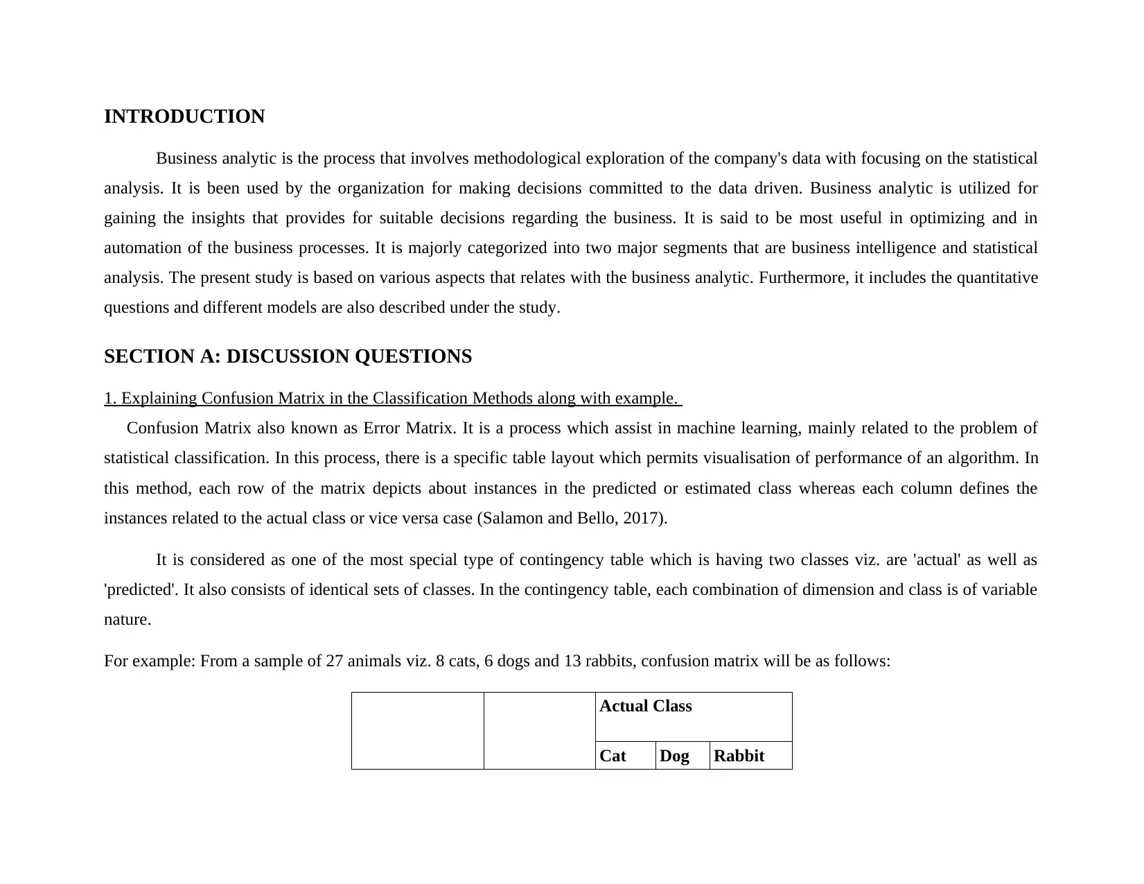
1. Explaining Confusion Matrix in the Classification Methods along with example.
Confusion Matrix also known as Error Matrix. It is a process which assist in machine learning, mainly related to the problem of
statistical classification. In this process, there is a specific table layout which permits visualisation of performance of an algorithm. In
this method, each row of the matrix depicts about instances in the predicted or estimated class whereas each column defines the
instances related to the actual class or vice versa case (Salamon and Bello, 2017).
It is considered as one of the most special type of contingency table which is having two classes viz. are 'actual' as well as
'predicted'. It also consists of identical sets of classes. In the contingency table, each combination of dimension and class is of variable
nature.
For example: From a sample of 27 animals viz. 8 cats, 6 dogs and 13 rabbits, confusion matrix will be as follows:
Actual Class
Cat Dog Rabbit
Business analytic is the process that involves methodological exploration of the company's data with focusing on the statistical
analysis. It is been used by the organization for making decisions committed to the data driven. Business analytic is utilized for
gaining the insights that provides for suitable decisions regarding the business. It is said to be most useful in optimizing and in
automation of the business processes. It is majorly categorized into two major segments that are business intelligence and statistical
analysis. The present study is based on various aspects that relates with the business analytic. Furthermore, it includes the quantitative
questions and different models are also described under the study.
SECTION A: DISCUSSION QUESTIONS
1. Explaining Confusion Matrix in the Classification Methods along with example.
Confusion Matrix also known as Error Matrix. It is a process which assist in machine learning, mainly related to the problem of
statistical classification. In this process, there is a specific table layout which permits visualisation of performance of an algorithm. In
this method, each row of the matrix depicts about instances in the predicted or estimated class whereas each column defines the
instances related to the actual class or vice versa case (Salamon and Bello, 2017).
It is considered as one of the most special type of contingency table which is having two classes viz. are 'actual' as well as
'predicted'. It also consists of identical sets of classes. In the contingency table, each combination of dimension and class is of variable
nature.
For example: From a sample of 27 animals viz. 8 cats, 6 dogs and 13 rabbits, confusion matrix will be as follows:
Actual Class
Cat Dog Rabbit
Paraphrase This Document
Need a fresh take? Get an instant paraphrase of this document with our AI Paraphraser
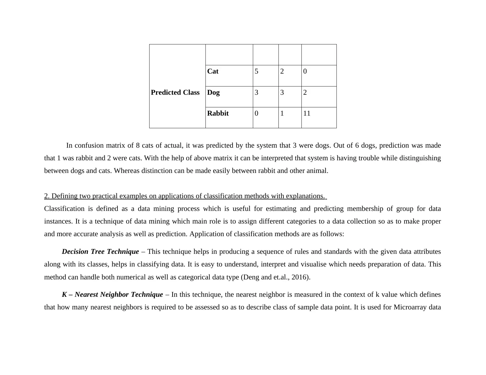
Predicted Class
Cat 5 2 0
Dog 3 3 2
Rabbit 0 1 11
In confusion matrix of 8 cats of actual, it was predicted by the system that 3 were dogs. Out of 6 dogs, prediction was made
that 1 was rabbit and 2 were cats. With the help of above matrix it can be interpreted that system is having trouble while distinguishing
between dogs and cats. Whereas distinction can be made easily between rabbit and other animal.
2. Defining two practical examples on applications of classification methods with explanations.
Classification is defined as a data mining process which is useful for estimating and predicting membership of group for data
instances. It is a technique of data mining which main role is to assign different categories to a data collection so as to make proper
and more accurate analysis as well as prediction. Application of classification methods are as follows:
Decision Tree Technique – This technique helps in producing a sequence of rules and standards with the given data attributes
along with its classes, helps in classifying data. It is easy to understand, interpret and visualise which needs preparation of data. This
method can handle both numerical as well as categorical data type (Deng and et.al., 2016).
K – Nearest Neighbor Technique – In this technique, the nearest neighbor is measured in the context of k value which defines
that how many nearest neighbors is required to be assessed so as to describe class of sample data point. It is used for Microarray data
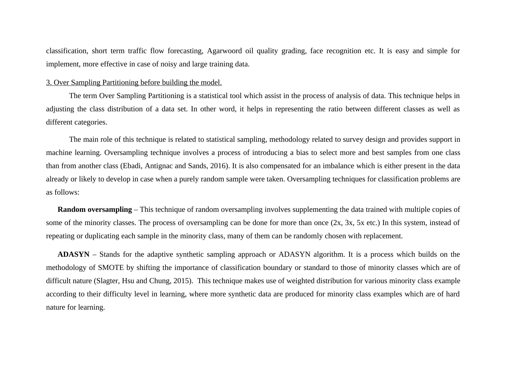
classification, short term traffic flow forecasting, Agarwoord oil quality grading, face recognition etc. It is easy and simple for
implement, more effective in case of noisy and large training data.
3. Over Sampling Partitioning before building the model.
The term Over Sampling Partitioning is a statistical tool which assist in the process of analysis of data. This technique helps in
adjusting the class distribution of a data set. In other word, it helps in representing the ratio between different classes as well as
different categories.
The main role of this technique is related to statistical sampling, methodology related to survey design and provides support in
machine learning. Oversampling technique involves a process of introducing a bias to select more and best samples from one class
than from another class (Ebadi, Antignac and Sands, 2016). It is also compensated for an imbalance which is either present in the data
already or likely to develop in case when a purely random sample were taken. Oversampling techniques for classification problems are
as follows:
Random oversampling – This technique of random oversampling involves supplementing the data trained with multiple copies of
some of the minority classes. The process of oversampling can be done for more than once (2x, 3x, 5x etc.) In this system, instead of
repeating or duplicating each sample in the minority class, many of them can be randomly chosen with replacement.
ADASYN – Stands for the adaptive synthetic sampling approach or ADASYN algorithm. It is a process which builds on the
methodology of SMOTE by shifting the importance of classification boundary or standard to those of minority classes which are of
difficult nature (Slagter, Hsu and Chung, 2015). This technique makes use of weighted distribution for various minority class example
according to their difficulty level in learning, where more synthetic data are produced for minority class examples which are of hard
nature for learning.
⊘ This is a preview!⊘
Do you want full access?
Subscribe today to unlock all pages.
Trusted by 1+ million students worldwide
4. Explaining how explanatory and categorical variables can be used in logistic regression
Logistic regression model is the appropriate technique for analysing and conducting the study for describing the data and for
effectively establishing the relationship between the dependent and the independent variable. It is also called as the predictive analysis
for evaluating the outcome. This resultant outcome is been measured under the model with the dichotomous variable. It is analysis that
is made for estimating the data value on the basis of the previous observations of data set. It has become a vital tool under the
discipline of learning. It is the approach that allows for using the algorithm for classifying the incoming data on the basis of historical
data. It is used for predicting the chance of winning or losing the situation in the future for any of the condition. A per the situation
given it is assumed that the two explanatory variable are been determined in the logistic regression model as the categorical variable
that is X1 and X2 where under X1 the categories are made as high, low and average while under X2 the classifications are made as
Sydney, Melbourne and Brisbane. These variables will be used as the dependent and the independent variable in the logistic regression
model. For example- The categorical variable that has low, high, average and the reference or the level of response variable is slow. In
case, the coefficient for the high resulted as 1.3, then the change in variable from the low to high raises natural log of odds of event by
the 1.3.
Paraphrase This Document
Need a fresh take? Get an instant paraphrase of this document with our AI Paraphraser
SECTION B: QUANTITATIVE QUESTIONS
5.
a. Explaining steps of KNN model in relation to making predictions about customers who will spend more than $1000
b. Developing a predictive model for making assessment about new female customer
6.
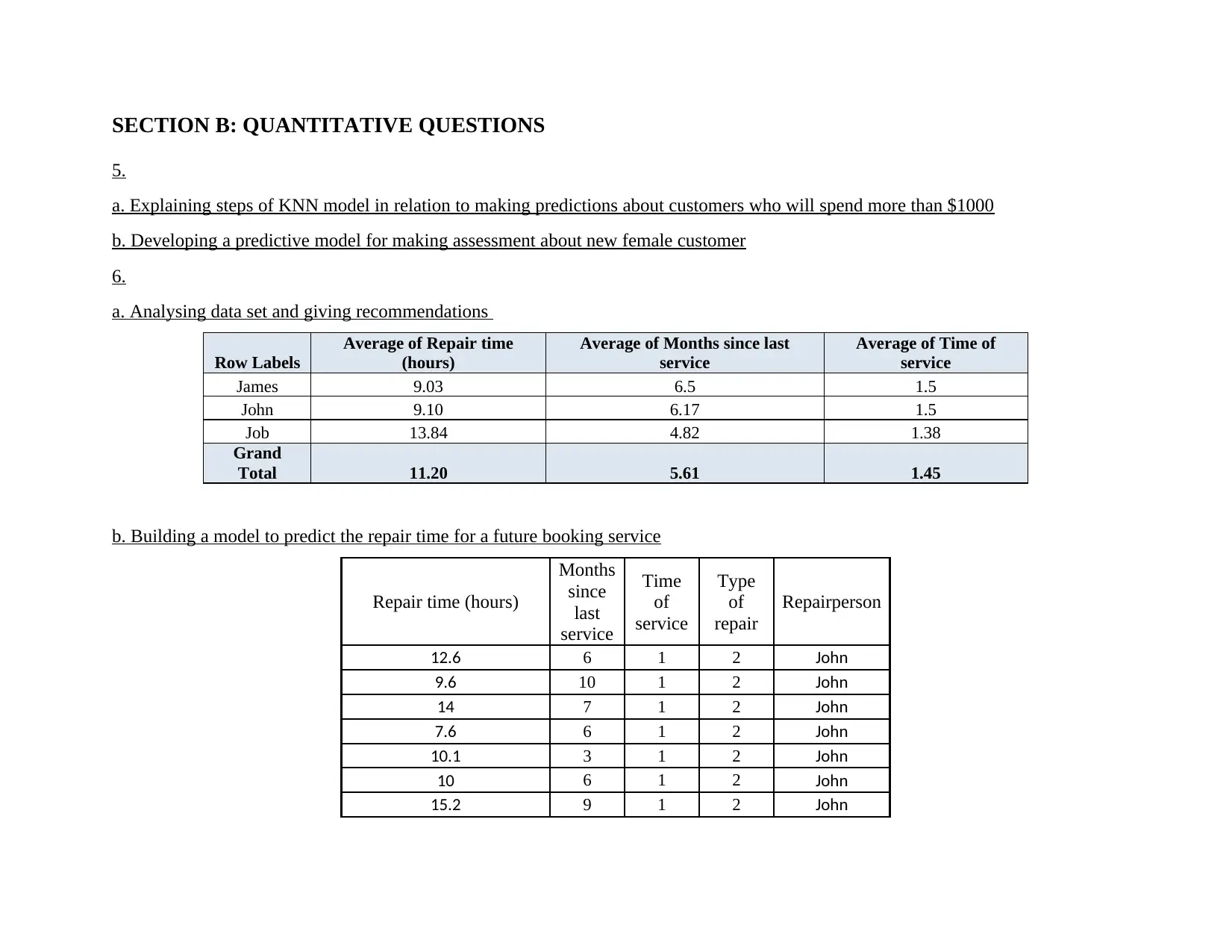
a. Analysing data set and giving recommendations
Row Labels
Average of Repair time
(hours)
Average of Months since last
service
Average of Time of
service
James 9.03 6.5 1.5
John 9.10 6.17 1.5
Job 13.84 4.82 1.38
Grand
Total 11.20 5.61 1.45
b. Building a model to predict the repair time for a future booking service
Repair time (hours)
Months
since
last
service
Time
of
service
Type
of
repair
Repairperson
12.6 6 1 2 John
9.6 10 1 2 John
14 7 1 2 John
7.6 6 1 2 John
10.1 3 1 2 John
10 6 1 2 John
15.2 9 1 2 John
5.
a. Explaining steps of KNN model in relation to making predictions about customers who will spend more than $1000
b. Developing a predictive model for making assessment about new female customer
6.
a. Analysing data set and giving recommendations
Row Labels
Average of Repair time
(hours)
Average of Months since last
service
Average of Time of
service
James 9.03 6.5 1.5
John 9.10 6.17 1.5
Job 13.84 4.82 1.38
Grand
Total 11.20 5.61 1.45
b. Building a model to predict the repair time for a future booking service
Repair time (hours)
Months
since
last
service
Time
of
service
Type
of
repair
Repairperson
12.6 6 1 2 John
9.6 10 1 2 John
14 7 1 2 John
7.6 6 1 2 John
10.1 3 1 2 John
10 6 1 2 John
15.2 9 1 2 John
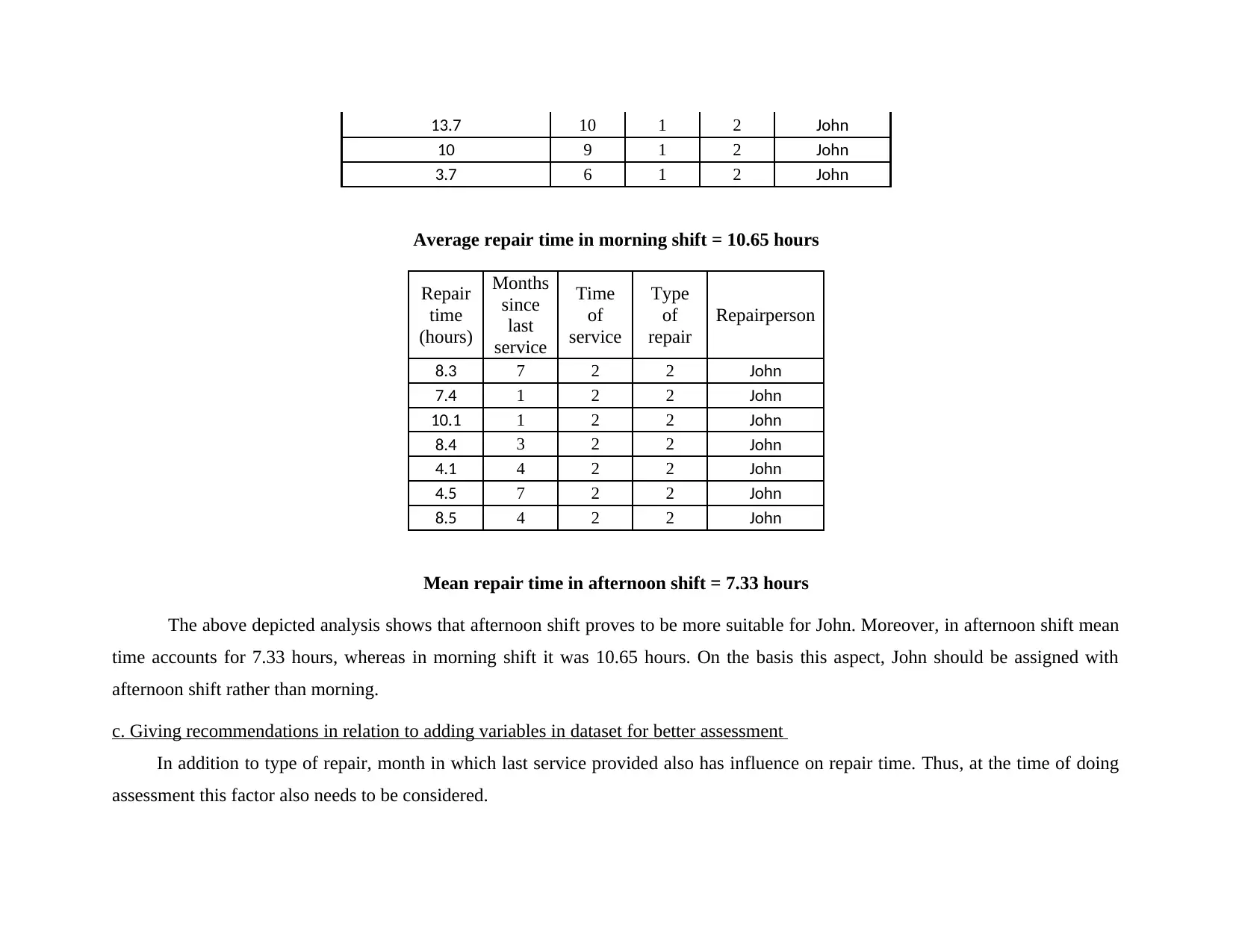
13.7 10 1 2 John
10 9 1 2 John
3.7 6 1 2 John
Average repair time in morning shift = 10.65 hours
Repair
time
(hours)
Months
since
last
service
Time
of
service
Type
of
repair
Repairperson
8.3 7 2 2 John
7.4 1 2 2 John
10.1 1 2 2 John
8.4 3 2 2 John
4.1 4 2 2 John
4.5 7 2 2 John
8.5 4 2 2 John
Mean repair time in afternoon shift = 7.33 hours
The above depicted analysis shows that afternoon shift proves to be more suitable for John. Moreover, in afternoon shift mean
time accounts for 7.33 hours, whereas in morning shift it was 10.65 hours. On the basis this aspect, John should be assigned with
afternoon shift rather than morning.
c. Giving recommendations in relation to adding variables in dataset for better assessment
In addition to type of repair, month in which last service provided also has influence on repair time. Thus, at the time of doing
assessment this factor also needs to be considered.
⊘ This is a preview!⊘
Do you want full access?
Subscribe today to unlock all pages.
Trusted by 1+ million students worldwide
7.
a. Explaining approach in relation to filling missing values in excel sheet
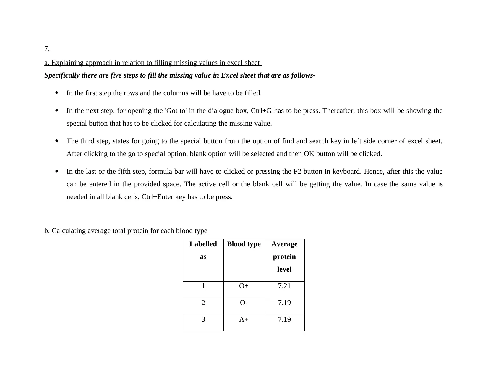
Specifically there are five steps to fill the missing value in Excel sheet that are as follows-
In the first step the rows and the columns will be have to be filled.
In the next step, for opening the 'Got to' in the dialogue box, Ctrl+G has to be press. Thereafter, this box will be showing the
special button that has to be clicked for calculating the missing value.
The third step, states for going to the special button from the option of find and search key in left side corner of excel sheet.
After clicking to the go to special option, blank option will be selected and then OK button will be clicked.
In the last or the fifth step, formula bar will have to clicked or pressing the F2 button in keyboard. Hence, after this the value
can be entered in the provided space. The active cell or the blank cell will be getting the value. In case the same value is
needed in all blank cells, Ctrl+Enter key has to be press.
b. Calculating average total protein for each blood type
Labelled
as
Blood type Average
protein
level
1 O+ 7.21
2 O- 7.19
3 A+ 7.19
a. Explaining approach in relation to filling missing values in excel sheet
Specifically there are five steps to fill the missing value in Excel sheet that are as follows-
In the first step the rows and the columns will be have to be filled.
In the next step, for opening the 'Got to' in the dialogue box, Ctrl+G has to be press. Thereafter, this box will be showing the
special button that has to be clicked for calculating the missing value.
The third step, states for going to the special button from the option of find and search key in left side corner of excel sheet.
After clicking to the go to special option, blank option will be selected and then OK button will be clicked.
In the last or the fifth step, formula bar will have to clicked or pressing the F2 button in keyboard. Hence, after this the value
can be entered in the provided space. The active cell or the blank cell will be getting the value. In case the same value is
needed in all blank cells, Ctrl+Enter key has to be press.
b. Calculating average total protein for each blood type
Labelled
as
Blood type Average
protein
level
1 O+ 7.21
2 O- 7.19
3 A+ 7.19
Paraphrase This Document
Need a fresh take? Get an instant paraphrase of this document with our AI Paraphraser
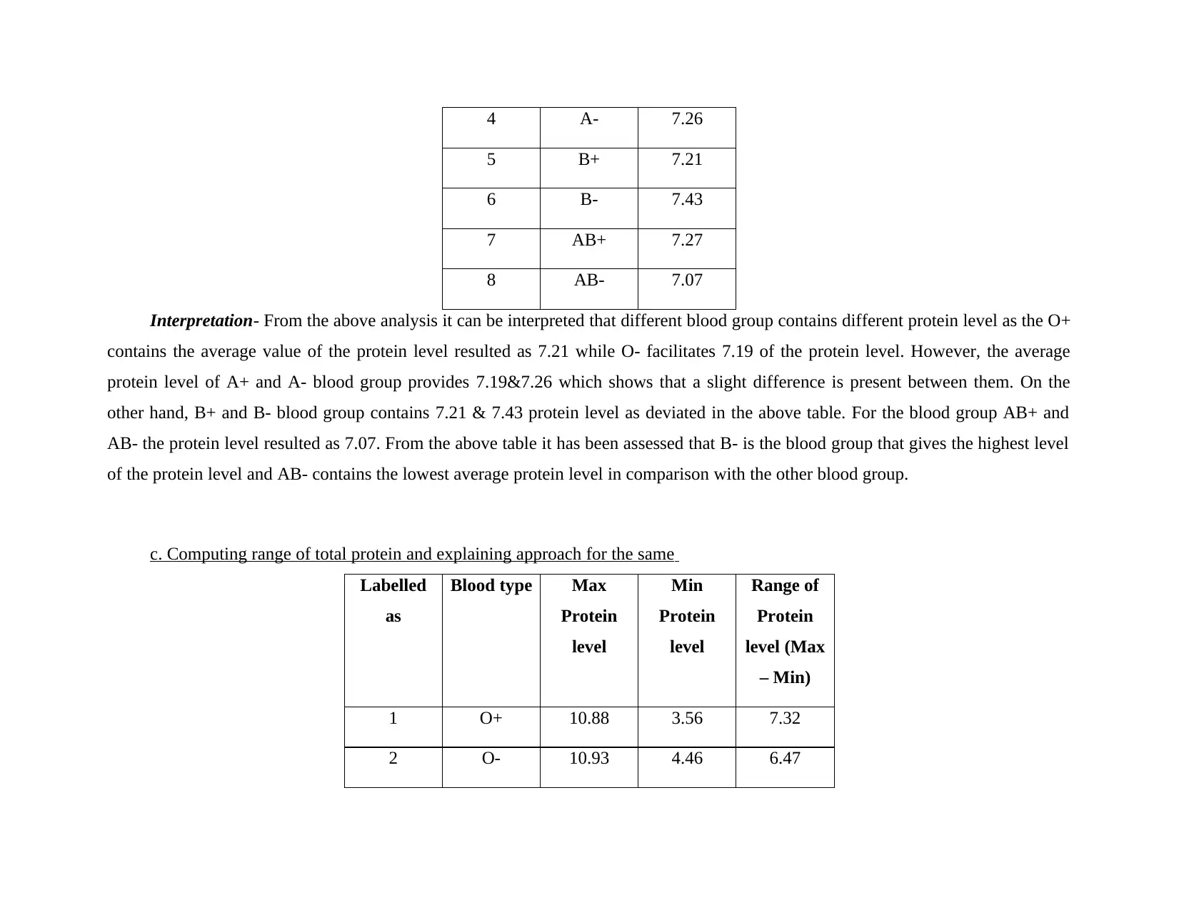
4 A- 7.26
5 B+ 7.21
6 B- 7.43
7 AB+ 7.27
8 AB- 7.07
Interpretation- From the above analysis it can be interpreted that different blood group contains different protein level as the O+
contains the average value of the protein level resulted as 7.21 while O- facilitates 7.19 of the protein level. However, the average
protein level of A+ and A- blood group provides 7.19&7.26 which shows that a slight difference is present between them. On the
other hand, B+ and B- blood group contains 7.21 & 7.43 protein level as deviated in the above table. For the blood group AB+ and
AB- the protein level resulted as 7.07. From the above table it has been assessed that B- is the blood group that gives the highest level
of the protein level and AB- contains the lowest average protein level in comparison with the other blood group.
c. Computing range of total protein and explaining approach for the same
Labelled
as
Blood type Max
Protein
level
Min
Protein
level
Range of
Protein
level (Max
– Min)
1 O+ 10.88 3.56 7.32
2 O- 10.93 4.46 6.47
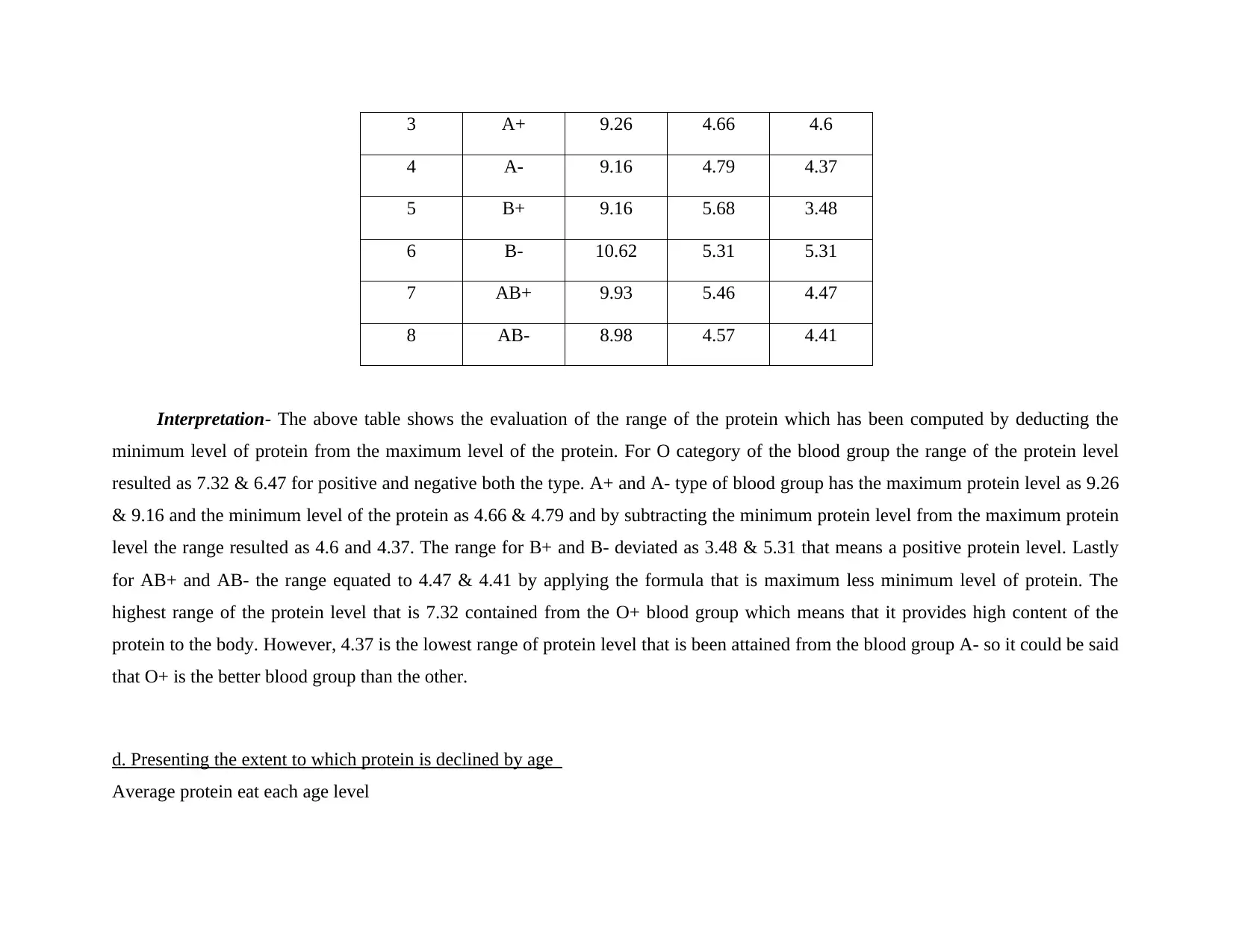
3 A+ 9.26 4.66 4.6
4 A- 9.16 4.79 4.37
5 B+ 9.16 5.68 3.48
6 B- 10.62 5.31 5.31
7 AB+ 9.93 5.46 4.47
8 AB- 8.98 4.57 4.41
Interpretation- The above table shows the evaluation of the range of the protein which has been computed by deducting the
minimum level of protein from the maximum level of the protein. For O category of the blood group the range of the protein level
resulted as 7.32 & 6.47 for positive and negative both the type. A+ and A- type of blood group has the maximum protein level as 9.26
& 9.16 and the minimum level of the protein as 4.66 & 4.79 and by subtracting the minimum protein level from the maximum protein
level the range resulted as 4.6 and 4.37. The range for B+ and B- deviated as 3.48 & 5.31 that means a positive protein level. Lastly
for AB+ and AB- the range equated to 4.47 & 4.41 by applying the formula that is maximum less minimum level of protein. The
highest range of the protein level that is 7.32 contained from the O+ blood group which means that it provides high content of the
protein to the body. However, 4.37 is the lowest range of protein level that is been attained from the blood group A- so it could be said
that O+ is the better blood group than the other.
d. Presenting the extent to which protein is declined by age
Average protein eat each age level
⊘ This is a preview!⊘
Do you want full access?
Subscribe today to unlock all pages.
Trusted by 1+ million students worldwide
1 out of 27
Related Documents


Your All-in-One AI-Powered Toolkit for Academic Success.
+13062052269
info@desklib.com
Available 24*7 on WhatsApp / Email
![[object Object]](/_next/static/media/star-bottom.7253800d.svg)
Unlock your academic potential
Copyright © 2020–2026 A2Z Services. All Rights Reserved. Developed and managed by ZUCOL.