Business Analytics and Statistics Research Report Analysis
VerifiedAdded on 2020/03/16
|17
|3234
|103
Report
AI Summary
This business analytics research report investigates sales performance, profit drivers, and cost optimization strategies for a business. The report begins with an introduction and problem definition, identifying the need to increase sales and decrease the cost of goods sold. It then outlines the analytical methods employed, including descriptive statistics, regression analysis, ANOVA, and t-tests using SPSS. The analysis explores key questions such as top/worst selling products, the impact of product location, differences in payment methods, seasonal sales variations, and the influence of rainfall and staff costs. Findings reveal insights into product performance, payment preferences, and factors affecting sales and profit. The report includes tables and figures summarizing the data analysis, providing a comprehensive overview of the business's performance and strategic recommendations for improvement.
Chapter: 1 Business Analytics and Statistics Research Report
Contents
Chapter: 1 Business Analytics and Statistics Research Report..............................................................1
1.1 Introduction.................................................................................................................................1
1.2 Definition of problem and the business intelligence required......................................................1
1.3 Analytics method selected for the research..................................................................................1
1.4 Scaling.........................................................................................................................................2
1.5 Descriptive analysis.....................................................................................................................3
1.6 What are the top/worst selling products in terms of sales?...........................................................5
1.7 There a difference in payments methods?....................................................................................7
1.8 Are the differences in sales performance based on where the product is located in the shop?
How does this affect both profits and revenue?.......................................................................................9
1.9 Is there a difference in sales and gross profits between different months of the year?...............11
1.10 Are their differences in sales performance between different seasons?.....................................11
1.11 Relationship between rainfall and profit....................................................................................13
1.12 Impact of Rainfall and Staff cost on sales..................................................................................13
1.13 Results from the analysis...........................................................................................................14
Paraphrase This Document
Need a fresh take? Get an instant paraphrase of this document with our AI Paraphraser
List of tables
Table 1 Descriptive statistics of the variables included in the data set.........................................................6
Table 2 Using ANOVA to test the difference in product location and sales.............................................10
Table 3 Multiple comparison results from the ANOVA table...................................................................11
Table 4 Using ANOVA table to show the results for difference in sales in month of the year..................12
Table 5 ANOVA table for season wise difference....................................................................................13
Table 6 Multiple comparison for season wise difference...........................................................................14
Table 7 Relationship between rainfall and profit.......................................................................................14
Table 8 Results from model summary.......................................................................................................15
Table 9 Results from ANOVA..................................................................................................................15
Table 10 Results from regression coefficients...........................................................................................15
List of figures
Figure 1 Variable in the data set and their scaling......................................................................................3
Figure 2 Variable in the data set and their scaling.......................................................................................4
Figure 3 finding the best and worst performers using the box plot.............................................................7
Figure 4 Low cost of goods sold and high sales products............................................................................8
Figure 5 Measuring difference in payment method from independent sample t test.................................10
1.1 Introduction
The main motive of every business is to maximize the profits. One can maximize the profit either
by increasing the revenue or by decreasing the cost of goods sold. Increase in the margin
between the price and the cost increases the profit.
1.2 Definition of problem and the business intelligence required
In this case the main challenge for the CEO is to increase the average sales of the product and at
the same time to decrease the cost of goods sold(Linof & Berry 2011; Chopra et al. 2011). Even
though the business has started only two years ago, it is important for the company to make
strategies to cut the cost and increase sales. With such problem in hand, this research will try to
find the answers to the following questions:
1. What are the top/worst selling products in terms of sales?
2. Are the differences in sales performance based on where the product is located in the
shop? How does this affect both profits and revenue?
3. Is there a difference in sales and gross profits between different months of the year?
4. Are their differences in sales performance between different seasons?
5. What is the impact of rainfall and the staff cost on the sales?
6. What is the impact of cost of goods sold and total sales on Net profit?
1.3 Analytics method selected for the research
On the basis of the research question proposed in the above section, different analytical
techniques have been used to find the answer. Data analysis was performed in Statistical Package
for Social Science (SPSS). The first step was to import the data into SPSS correctly and scale
them properly. Apart from that various other statistical techniques such as regression analysis,
correlation, ANOVA test, and independent t test and descriptive analysis has also been
performed(Easterby-Smith et al. 2008; Creswell 2003; Rajasekar et al. 2013). In the first section
the scaling and the descriptive analysis have been performed followed by other statistical tests.
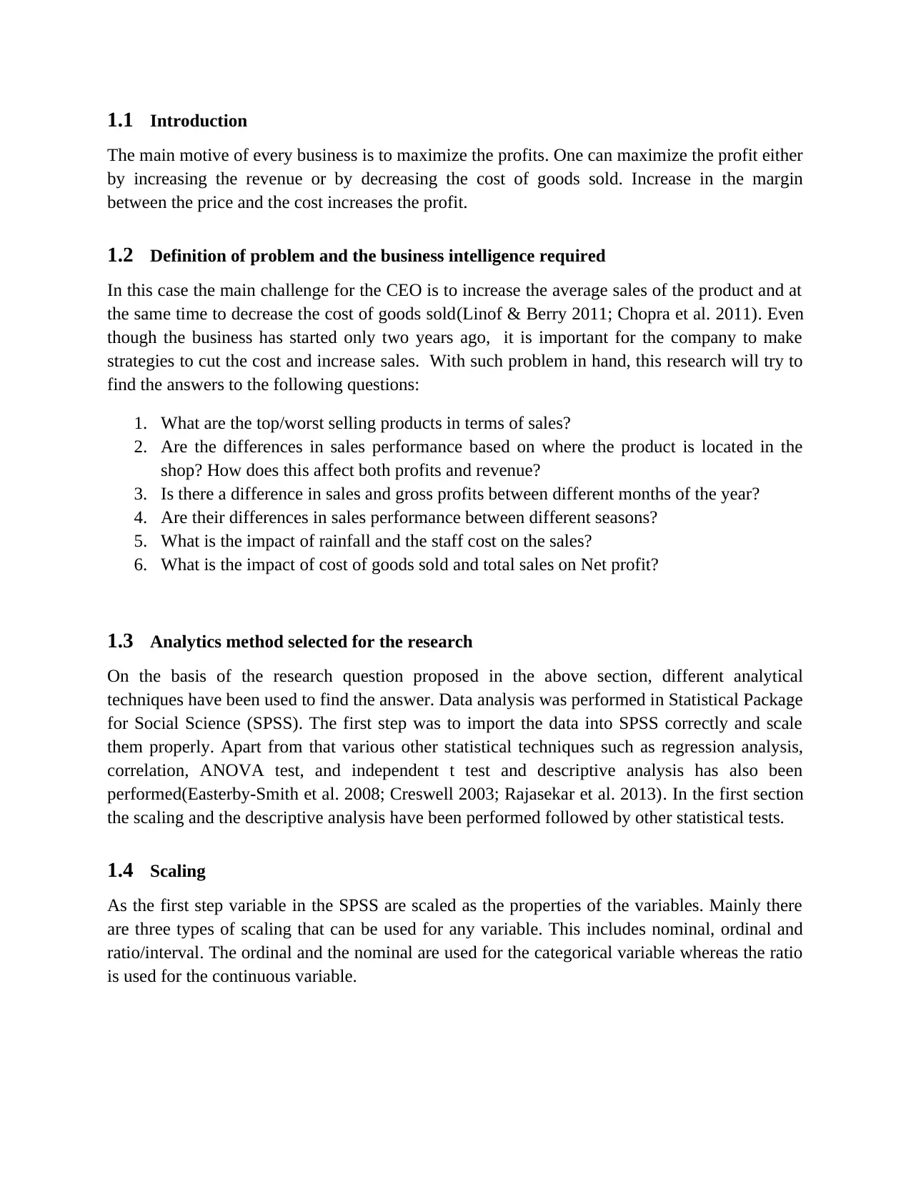
1.4 Scaling
As the first step variable in the SPSS are scaled as the properties of the variables. Mainly there
are three types of scaling that can be used for any variable. This includes nominal, ordinal and
ratio/interval. The ordinal and the nominal are used for the categorical variable whereas the ratio
is used for the continuous variable.
The main motive of every business is to maximize the profits. One can maximize the profit either
by increasing the revenue or by decreasing the cost of goods sold. Increase in the margin
between the price and the cost increases the profit.
1.2 Definition of problem and the business intelligence required
In this case the main challenge for the CEO is to increase the average sales of the product and at
the same time to decrease the cost of goods sold(Linof & Berry 2011; Chopra et al. 2011). Even
though the business has started only two years ago, it is important for the company to make
strategies to cut the cost and increase sales. With such problem in hand, this research will try to
find the answers to the following questions:
1. What are the top/worst selling products in terms of sales?
2. Are the differences in sales performance based on where the product is located in the
shop? How does this affect both profits and revenue?
3. Is there a difference in sales and gross profits between different months of the year?
4. Are their differences in sales performance between different seasons?
5. What is the impact of rainfall and the staff cost on the sales?
6. What is the impact of cost of goods sold and total sales on Net profit?
1.3 Analytics method selected for the research
On the basis of the research question proposed in the above section, different analytical
techniques have been used to find the answer. Data analysis was performed in Statistical Package
for Social Science (SPSS). The first step was to import the data into SPSS correctly and scale
them properly. Apart from that various other statistical techniques such as regression analysis,
correlation, ANOVA test, and independent t test and descriptive analysis has also been
performed(Easterby-Smith et al. 2008; Creswell 2003; Rajasekar et al. 2013). In the first section
the scaling and the descriptive analysis have been performed followed by other statistical tests.
1.4 Scaling
As the first step variable in the SPSS are scaled as the properties of the variables. Mainly there
are three types of scaling that can be used for any variable. This includes nominal, ordinal and
ratio/interval. The ordinal and the nominal are used for the categorical variable whereas the ratio
is used for the continuous variable.
⊘ This is a preview!⊘
Do you want full access?
Subscribe today to unlock all pages.
Trusted by 1+ million students worldwide
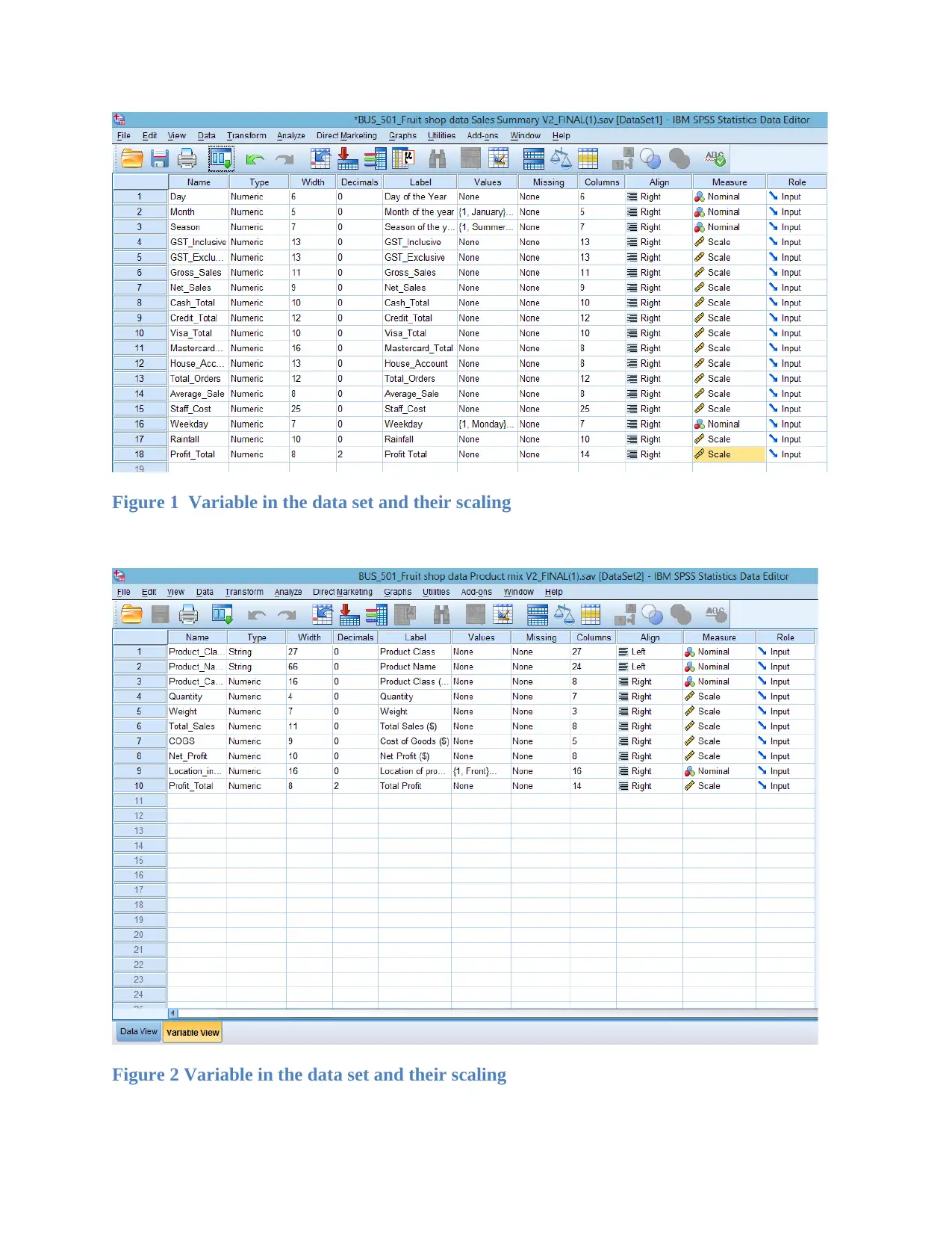
Figure 1 Variable in the data set and their scaling
Figure 2 Variable in the data set and their scaling
Figure 2 Variable in the data set and their scaling
Paraphrase This Document
Need a fresh take? Get an instant paraphrase of this document with our AI Paraphraser
Initially the scale of the variables such as the season of the year, day of the week and month of
the year was scaled as ordinal. However the correct scaling of those variables is nominal as there
is no proper hierarchy of these variables. In other words it cannot be said that Monday is greater
than Tuesday or the March is greater than April etc. So the scale of such variables has been
changed.
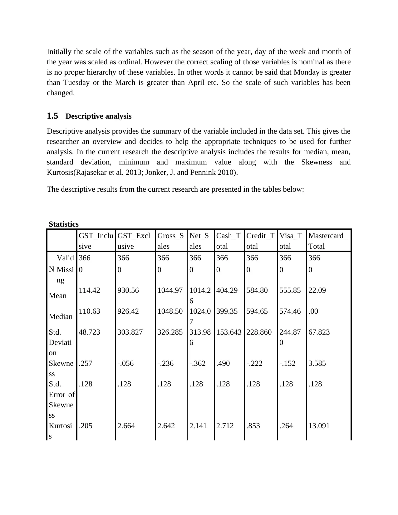
1.5 Descriptive analysis
Descriptive analysis provides the summary of the variable included in the data set. This gives the
researcher an overview and decides to help the appropriate techniques to be used for further
analysis. In the current research the descriptive analysis includes the results for median, mean,
standard deviation, minimum and maximum value along with the Skewness and
Kurtosis(Rajasekar et al. 2013; Jonker, J. and Pennink 2010).
The descriptive results from the current research are presented in the tables below:
Statistics
GST_Inclu
sive
GST_Excl
usive
Gross_S
ales
Net_S
ales
Cash_T
otal
Credit_T
otal
Visa_T
otal
Mastercard_
Total
N
Valid 366 366 366 366 366 366 366 366
Missi
ng
0 0 0 0 0 0 0 0
Mean 114.42 930.56 1044.97 1014.2
6
404.29 584.80 555.85 22.09
Median 110.63 926.42 1048.50 1024.0
7
399.35 594.65 574.46 .00
Std.
Deviati
on
48.723 303.827 326.285 313.98
6
153.643 228.860 244.87
0
67.823
Skewne
ss
.257 -.056 -.236 -.362 .490 -.222 -.152 3.585
Std.
Error of
Skewne
ss
.128 .128 .128 .128 .128 .128 .128 .128
Kurtosi
s
.205 2.664 2.642 2.141 2.712 .853 .264 13.091
the year was scaled as ordinal. However the correct scaling of those variables is nominal as there
is no proper hierarchy of these variables. In other words it cannot be said that Monday is greater
than Tuesday or the March is greater than April etc. So the scale of such variables has been
changed.
1.5 Descriptive analysis
Descriptive analysis provides the summary of the variable included in the data set. This gives the
researcher an overview and decides to help the appropriate techniques to be used for further
analysis. In the current research the descriptive analysis includes the results for median, mean,
standard deviation, minimum and maximum value along with the Skewness and
Kurtosis(Rajasekar et al. 2013; Jonker, J. and Pennink 2010).
The descriptive results from the current research are presented in the tables below:
Statistics
GST_Inclu
sive
GST_Excl
usive
Gross_S
ales
Net_S
ales
Cash_T
otal
Credit_T
otal
Visa_T
otal
Mastercard_
Total
N
Valid 366 366 366 366 366 366 366 366
Missi
ng
0 0 0 0 0 0 0 0
Mean 114.42 930.56 1044.97 1014.2
6
404.29 584.80 555.85 22.09
Median 110.63 926.42 1048.50 1024.0
7
399.35 594.65 574.46 .00
Std.
Deviati
on
48.723 303.827 326.285 313.98
6
153.643 228.860 244.87
0
67.823
Skewne
ss
.257 -.056 -.236 -.362 .490 -.222 -.152 3.585
Std.
Error of
Skewne
ss
.128 .128 .128 .128 .128 .128 .128 .128
Kurtosi
s
.205 2.664 2.642 2.141 2.712 .853 .264 13.091
Std.
Error of
Kurtosi
s
.254 .254 .254 .254 .254 .254 .254 .254
Minimu
m
0 0 0 0 0 0 0 0
Maxim
um
271 2492 2642 2370 1195 1407 1407 399
Statistics
House_Accou
nt
Total_Order
s
Average_Sal
e
Staff_Cost Rainfall Profit
Total
N Valid 366 366 358 366 365 366
Missing 0 0 8 0 1 0
Mean 37.39 55.54 18.52 248.69 3.98 30.7098
Median .00 56.00 18.31 247.19 .00 25.0300
Std. Deviation 113.204 15.844 3.985 52.418 9.811 30.05661
Skewness 5.280 -.568 3.758 .475 3.421 3.274
Std. Error of
Skewness
.128 .128 .129 .128 .128 .128
Kurtosis 39.983 3.470 35.684 -.576 12.600 18.572
Std. Error of Kurtosis .254 .254 .257 .254 .255 .254
Minimum -264 0 8 170 0 -33.98
Maximum 1113 129 61 351 63 271.97
Statistics
Quantity Total Sales
($)
Cost of
Goods ($)
Net Profit
($)
Total
Profit
N Valid 1034 1034 1034 1034 1034
Missing 0 0 0 0 0
Mean 71.90 369.96 205.22 164.74 164.7338
Median 12.00 85.15 49.55 35.02 35.0150
Std. Deviation 212.400 1014.719 561.072 482.106 482.10651
Skewness 8.205 8.511 8.325 9.234 9.234
Std. Error of
Skewness
.076 .076 .076 .076 .076
Kurtosis 104.538 105.970 97.171 126.885 126.884
⊘ This is a preview!⊘
Do you want full access?
Subscribe today to unlock all pages.
Trusted by 1+ million students worldwide
Std. Error of
Kurtosis
.152 .152 .152 .152 .152
Minimum 1 0 0 0 .00
Maximum 3769 17276 8573 8703 8702.93
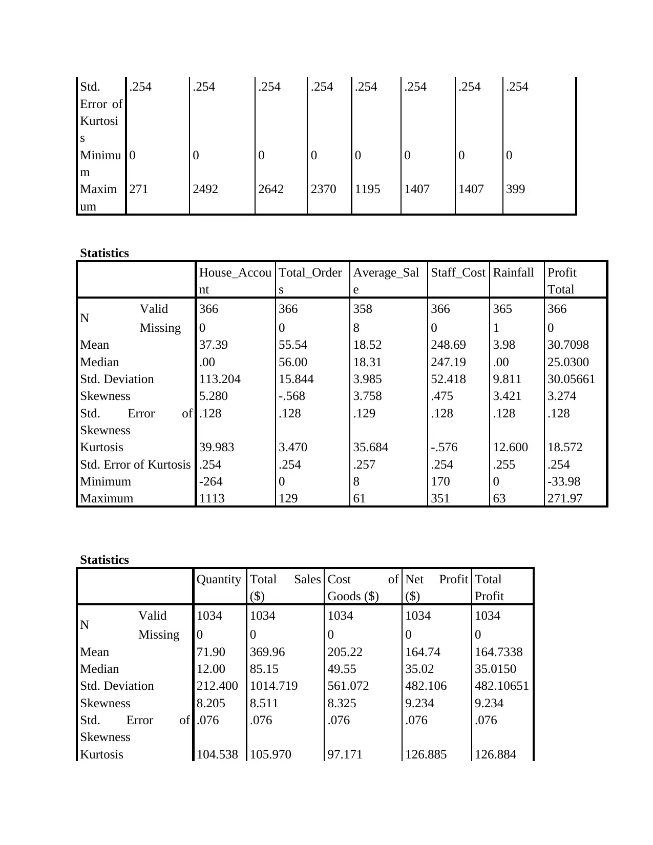
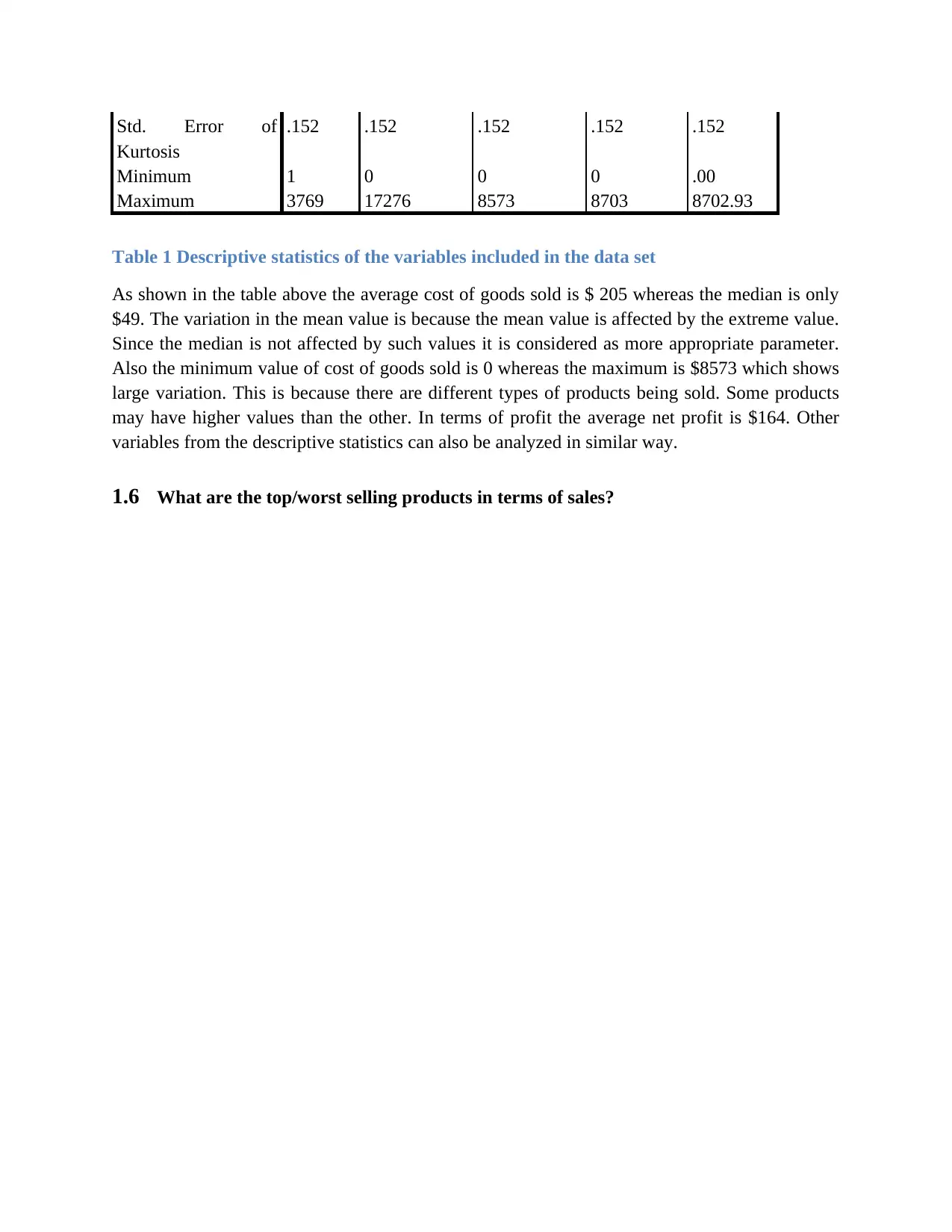
Table 1 Descriptive statistics of the variables included in the data set
As shown in the table above the average cost of goods sold is $ 205 whereas the median is only
$49. The variation in the mean value is because the mean value is affected by the extreme value.
Since the median is not affected by such values it is considered as more appropriate parameter.
Also the minimum value of cost of goods sold is 0 whereas the maximum is $8573 which shows
large variation. This is because there are different types of products being sold. Some products
may have higher values than the other. In terms of profit the average net profit is $164. Other
variables from the descriptive statistics can also be analyzed in similar way.
1.6 What are the top/worst selling products in terms of sales?
Kurtosis
.152 .152 .152 .152 .152
Minimum 1 0 0 0 .00
Maximum 3769 17276 8573 8703 8702.93
Table 1 Descriptive statistics of the variables included in the data set
As shown in the table above the average cost of goods sold is $ 205 whereas the median is only
$49. The variation in the mean value is because the mean value is affected by the extreme value.
Since the median is not affected by such values it is considered as more appropriate parameter.
Also the minimum value of cost of goods sold is 0 whereas the maximum is $8573 which shows
large variation. This is because there are different types of products being sold. Some products
may have higher values than the other. In terms of profit the average net profit is $164. Other
variables from the descriptive statistics can also be analyzed in similar way.
1.6 What are the top/worst selling products in terms of sales?
Paraphrase This Document
Need a fresh take? Get an instant paraphrase of this document with our AI Paraphraser
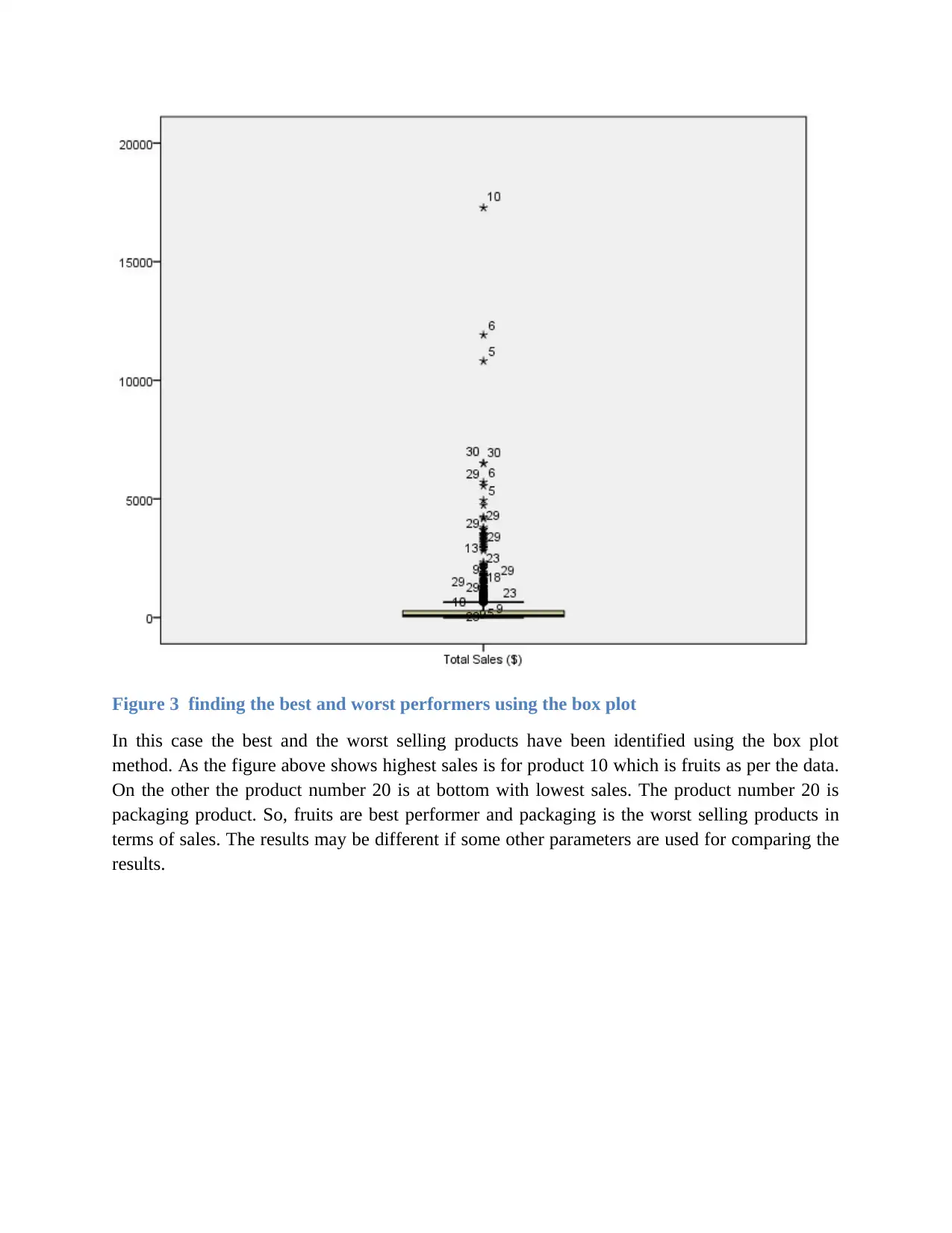
Figure 3 finding the best and worst performers using the box plot
In this case the best and the worst selling products have been identified using the box plot
method. As the figure above shows highest sales is for product 10 which is fruits as per the data.
On the other the product number 20 is at bottom with lowest sales. The product number 20 is
packaging product. So, fruits are best performer and packaging is the worst selling products in
terms of sales. The results may be different if some other parameters are used for comparing the
results.
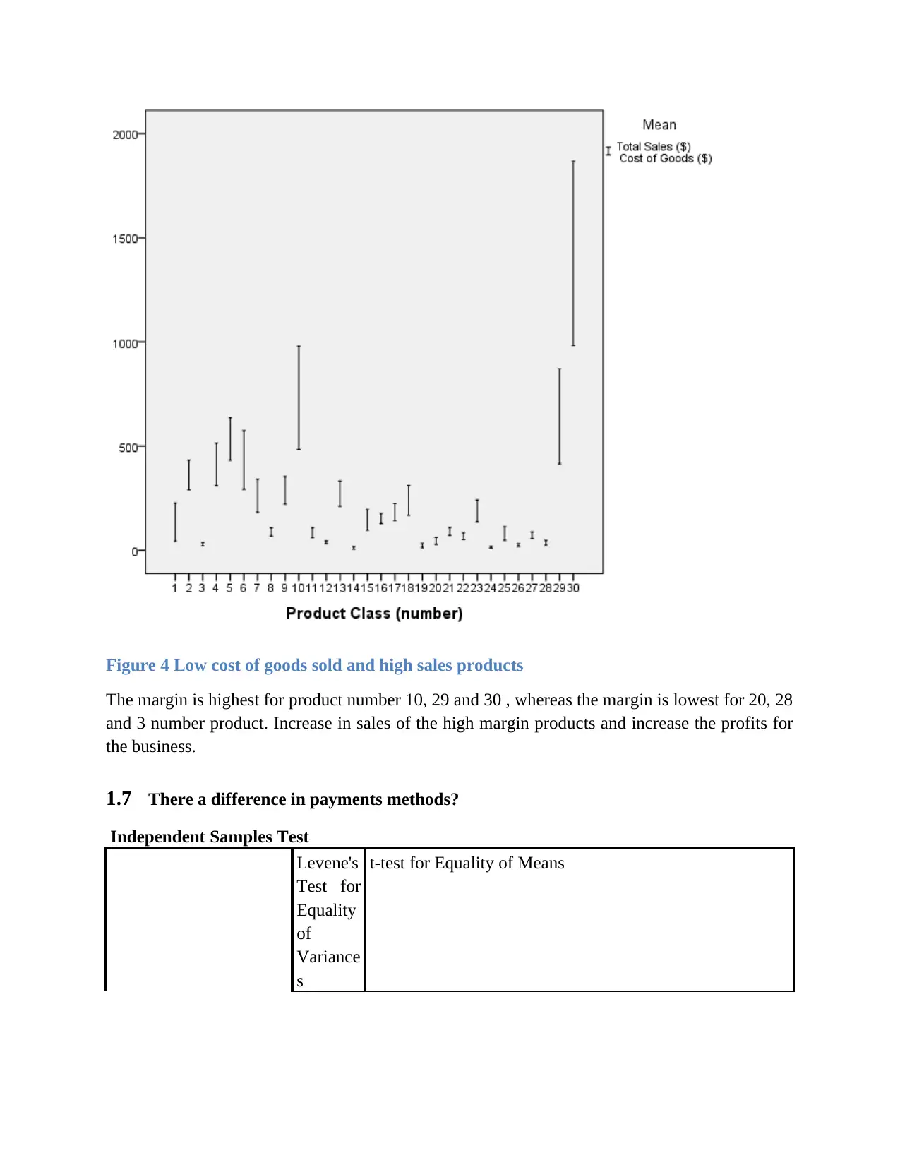
Figure 4 Low cost of goods sold and high sales products
The margin is highest for product number 10, 29 and 30 , whereas the margin is lowest for 20, 28
and 3 number product. Increase in sales of the high margin products and increase the profits for
the business.
1.7 There a difference in payments methods?
Independent Samples Test
Levene's
Test for
Equality
of
Variance
s
t-test for Equality of Means
⊘ This is a preview!⊘
Do you want full access?
Subscribe today to unlock all pages.
Trusted by 1+ million students worldwide
F Sig
.
t df Sig.
(2-
tailed
)
Mean
Differen
ce
Std.
Error
Differen
ce
95%
Confidence
Interval of the
Difference
Lower Upper
Cash_Total
Equal
varianc
es
assume
d
.00
1
.98
0
10.76
5
364 .000 150.910 14.018 123.34
3
178.47
8
Equal
varianc
es not
assume
d
10.77
9
363.33
9
.000 150.910 14.000 123.37
9
178.44
2
Credit_Total
Equal
varianc
es
assume
d
.71
4
.39
9
15.49
9
364 .000 288.419 18.609 251.82
4
325.01
5
Equal
varianc
es not
assume
d
15.56
9
363.38
9
.000 288.419 18.526 251.98
8
324.85
0
Visa_Total
Equal
varianc
es
assume
d
.05
9
.80
8
14.65
2
364 .000 298.101 20.346 258.09
1
338.11
1
Equal
varianc
es not
assume
d
14.72
7
362.79
2
.000 298.101 20.241 258.29
6
337.90
7
Paraphrase This Document
Need a fresh take? Get an instant paraphrase of this document with our AI Paraphraser
Mastercard_To
tal
Equal
varianc
es
assume
d
.53
3
.46
6
-.733 364 .464 -5.207 7.100 -
19.169
8.756
Equal
varianc
es not
assume
d
-.739 357.03
5
.460 -5.207 7.042 -
19.055
8.642
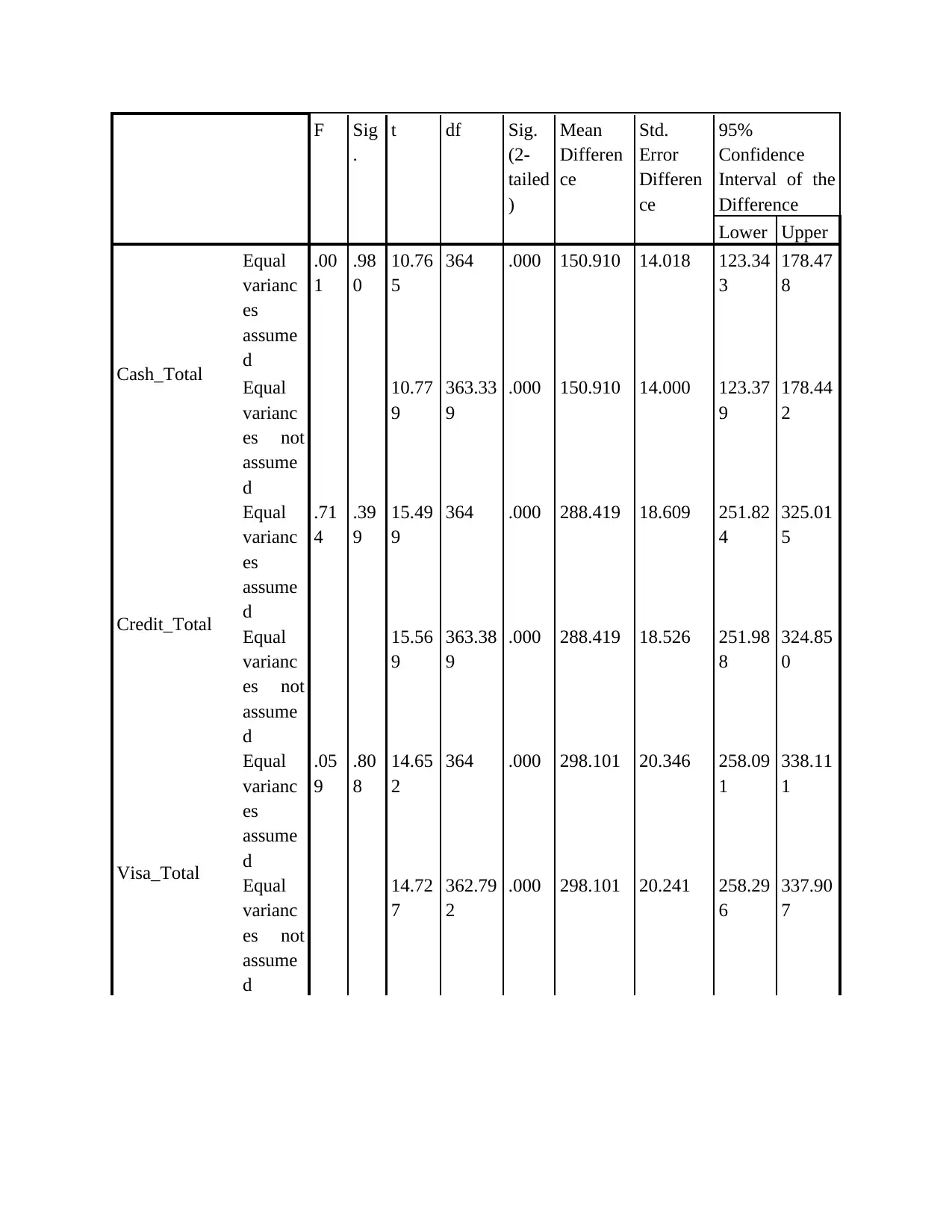
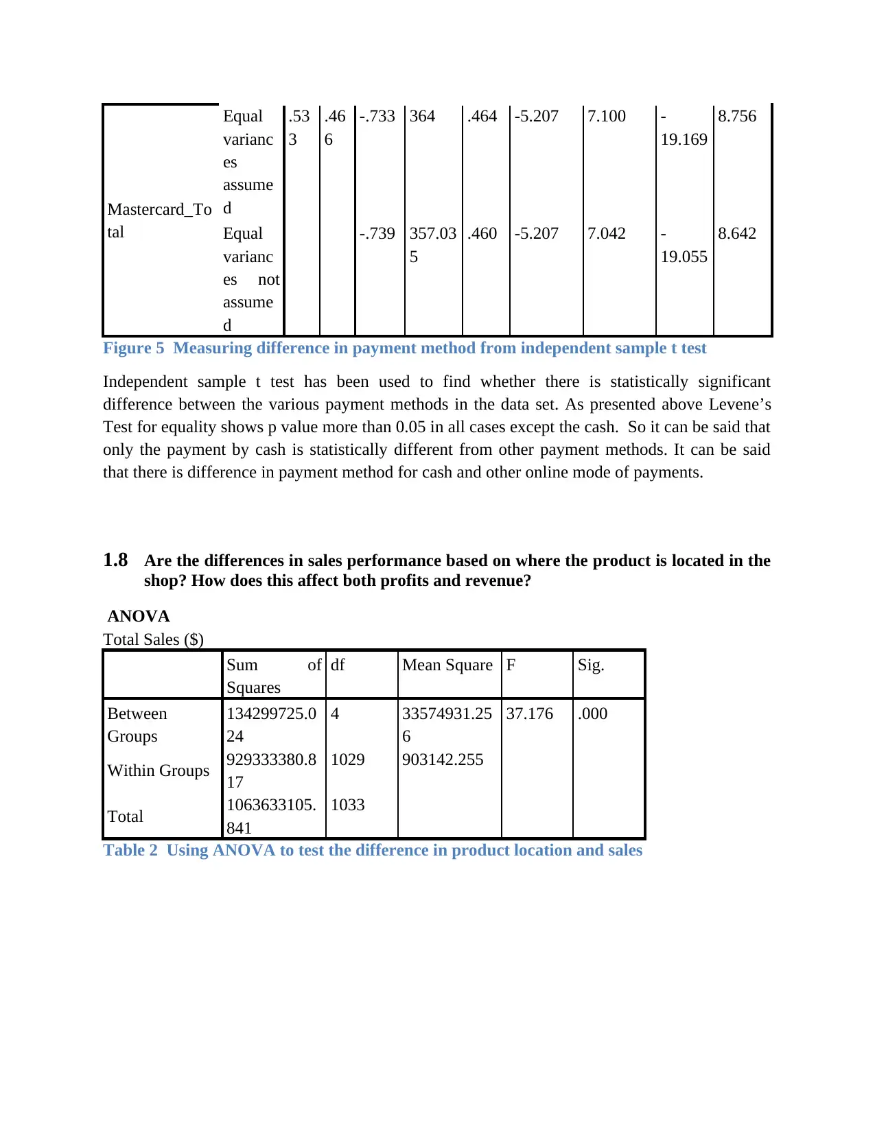
Figure 5 Measuring difference in payment method from independent sample t test
Independent sample t test has been used to find whether there is statistically significant
difference between the various payment methods in the data set. As presented above Levene’s
Test for equality shows p value more than 0.05 in all cases except the cash. So it can be said that
only the payment by cash is statistically different from other payment methods. It can be said
that there is difference in payment method for cash and other online mode of payments.
1.8 Are the differences in sales performance based on where the product is located in the
shop? How does this affect both profits and revenue?
ANOVA
Total Sales ($)
Sum of
Squares
df Mean Square F Sig.
Between
Groups
134299725.0
24
4 33574931.25
6
37.176 .000
Within Groups 929333380.8
17
1029 903142.255
Total 1063633105.
841
1033
Table 2 Using ANOVA to test the difference in product location and sales
tal
Equal
varianc
es
assume
d
.53
3
.46
6
-.733 364 .464 -5.207 7.100 -
19.169
8.756
Equal
varianc
es not
assume
d
-.739 357.03
5
.460 -5.207 7.042 -
19.055
8.642
Figure 5 Measuring difference in payment method from independent sample t test
Independent sample t test has been used to find whether there is statistically significant
difference between the various payment methods in the data set. As presented above Levene’s
Test for equality shows p value more than 0.05 in all cases except the cash. So it can be said that
only the payment by cash is statistically different from other payment methods. It can be said
that there is difference in payment method for cash and other online mode of payments.
1.8 Are the differences in sales performance based on where the product is located in the
shop? How does this affect both profits and revenue?
ANOVA
Total Sales ($)
Sum of
Squares
df Mean Square F Sig.
Between
Groups
134299725.0
24
4 33574931.25
6
37.176 .000
Within Groups 929333380.8
17
1029 903142.255
Total 1063633105.
841
1033
Table 2 Using ANOVA to test the difference in product location and sales
Multiple Comparisons
Dependent Variable: Total Sales ($)
Bonferroni
(I) Location of
product in shop
(J) Location of
product in shop
Mean
Difference
(I-J)
Std.
Error
Sig. 95% Confidence
Interval
Lower
Bound
Upper
Bound
Front
Left 354.531* 90.712 .001 99.35 609.71
Outside Front -2811.617* 284.761 .000 -3612.68 -2010.56
Rear 36.679 104.135 1.000 -256.26 329.62
Right 332.860* 93.438 .004 70.01 595.71
Left
Front -354.531* 90.712 .001 -609.71 -99.35
Outside Front -3166.148* 278.682 .000 -3950.11 -2382.19
Rear -317.851* 86.136 .002 -560.16 -75.54
Right -21.671 72.842 1.000 -226.58 183.24
Outside Front
Front 2811.617* 284.761 .000 2010.56 3612.68
Left 3166.148* 278.682 .000 2382.19 3950.11
Rear 2848.297* 283.336 .000 2051.24 3645.35
Right 3144.477* 279.582 .000 2357.99 3930.97
Rear
Front -36.679 104.135 1.000 -329.62 256.26
Left 317.851* 86.136 .002 75.54 560.16
Outside Front -2848.297* 283.336 .000 -3645.35 -2051.24
Right 296.181* 89.003 .009 45.81 546.55
Right
Front -332.860* 93.438 .004 -595.71 -70.01
Left 21.671 72.842 1.000 -183.24 226.58
Outside Front -3144.477* 279.582 .000 -3930.97 -2357.99
Rear -296.181* 89.003 .009 -546.55 -45.81
*. The mean difference is significant at the 0.05 level.
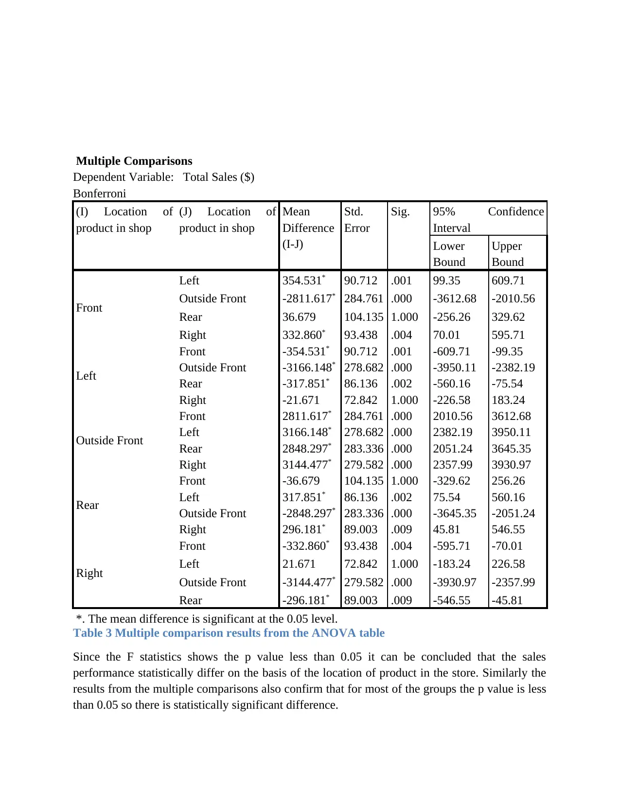
Table 3 Multiple comparison results from the ANOVA table
Since the F statistics shows the p value less than 0.05 it can be concluded that the sales
performance statistically differ on the basis of the location of product in the store. Similarly the
results from the multiple comparisons also confirm that for most of the groups the p value is less
than 0.05 so there is statistically significant difference.
Dependent Variable: Total Sales ($)
Bonferroni
(I) Location of
product in shop
(J) Location of
product in shop
Mean
Difference
(I-J)
Std.
Error
Sig. 95% Confidence
Interval
Lower
Bound
Upper
Bound
Front
Left 354.531* 90.712 .001 99.35 609.71
Outside Front -2811.617* 284.761 .000 -3612.68 -2010.56
Rear 36.679 104.135 1.000 -256.26 329.62
Right 332.860* 93.438 .004 70.01 595.71
Left
Front -354.531* 90.712 .001 -609.71 -99.35
Outside Front -3166.148* 278.682 .000 -3950.11 -2382.19
Rear -317.851* 86.136 .002 -560.16 -75.54
Right -21.671 72.842 1.000 -226.58 183.24
Outside Front
Front 2811.617* 284.761 .000 2010.56 3612.68
Left 3166.148* 278.682 .000 2382.19 3950.11
Rear 2848.297* 283.336 .000 2051.24 3645.35
Right 3144.477* 279.582 .000 2357.99 3930.97
Rear
Front -36.679 104.135 1.000 -329.62 256.26
Left 317.851* 86.136 .002 75.54 560.16
Outside Front -2848.297* 283.336 .000 -3645.35 -2051.24
Right 296.181* 89.003 .009 45.81 546.55
Right
Front -332.860* 93.438 .004 -595.71 -70.01
Left 21.671 72.842 1.000 -183.24 226.58
Outside Front -3144.477* 279.582 .000 -3930.97 -2357.99
Rear -296.181* 89.003 .009 -546.55 -45.81
*. The mean difference is significant at the 0.05 level.
Table 3 Multiple comparison results from the ANOVA table
Since the F statistics shows the p value less than 0.05 it can be concluded that the sales
performance statistically differ on the basis of the location of product in the store. Similarly the
results from the multiple comparisons also confirm that for most of the groups the p value is less
than 0.05 so there is statistically significant difference.
⊘ This is a preview!⊘
Do you want full access?
Subscribe today to unlock all pages.
Trusted by 1+ million students worldwide
1 out of 17
Related Documents


Your All-in-One AI-Powered Toolkit for Academic Success.
+13062052269
info@desklib.com
Available 24*7 on WhatsApp / Email
![[object Object]](/_next/static/media/star-bottom.7253800d.svg)
Unlock your academic potential
Copyright © 2020–2026 A2Z Services. All Rights Reserved. Developed and managed by ZUCOL.