Melbourne Campus BUS501: Business Analytics and Stats Research Report
VerifiedAdded on 2023/06/04
|27
|4777
|498
Report
AI Summary
This research report analyzes the performance of Honeybee Fruit, addressing key business questions for the CEO. The study examines product sales, identifying top and bottom performers, and investigates differences in payment methods (cash vs. credit). It assesses the impact of product location within the shop on sales, profits, and revenue, utilizing ANOVA tests to compare sales performance across different locations. The report further explores sales and gross profit variations across months and seasons, employing ANOVA to identify significant trends. The findings reveal that water and fruits are the best-selling products, and credit payments generate higher revenue than cash. Products located outside the front of the shop have the highest sales. The analysis also provides recommendations to the CEO based on these findings, aiming to optimize sales strategies, improve revenue, and address cost-related challenges. The report concludes with a discussion of the results and provides actionable insights to improve the business's performance.
BUS501 - Business Analytics and Statistics
Research Report
Melbourne Campus Instructions
21st September 2018
Research Report
Melbourne Campus Instructions
21st September 2018
Paraphrase This Document
Need a fresh take? Get an instant paraphrase of this document with our AI Paraphraser
Table of Contents
Introduction......................................................................................................................................4
Problem definition and business intelligence required....................................................................4
Results of the selected analytics methods and technical analysis....................................................5
What are the best and worst selling products in terms of sales?..................................................5
Is there a difference in payments methods? (Cash vs Credit)?....................................................6
Are the differences in sales performance based on where the product is located in the shop?
How does this effect both profits and revenue?...........................................................................8
Is there a difference in sales and gross profits between different months of the year?................9
Are their differences in sales performance between different seasons?....................................13
Discussion of the results and recommendations............................................................................14
Recommendations......................................................................................................................15
References......................................................................................................................................16
Appendix........................................................................................................................................17
List of tables
Table 1: Top best-selling products in terms of sales.......................................................................6
Table 2: Bottom 5 worst selling products in terms of sales.............................................................6
Table 3: Group Statistics.................................................................................................................7
Table 4: Independent Samples Test.................................................................................................7
Table 5: Descriptive statistics..........................................................................................................8
Table 6: ANOVA.............................................................................................................................8
Table 7: Descriptive statistics..........................................................................................................9
Table 8: ANOVA Table.................................................................................................................10
Table 9: Descriptive Statistics.......................................................................................................11
Table 10: ANOVA Table...............................................................................................................12
Table 12: Descriptive statistics......................................................................................................13
Table 13: ANOVA table................................................................................................................13
List of figures
Figure 1: Mean plot for gross sales versus month.........................................................................10
Figure 2: Mean plot for gross profits versus month......................................................................12
Figure 3: Mean plot for gross sales versus season of the year.......................................................14
⊘ This is a preview!⊘
Do you want full access?
Subscribe today to unlock all pages.
Trusted by 1+ million students worldwide
Introduction
Company sales is one of the key performances that shows that the business is either doing well
or in some verge to collapse. The CEO of Honeybee Fruit is a concerned person and would want
to understand how the company is performing. He is particularly interested in knowing which of
the products are doing well and which ones are not doing well in the market. With this in mind,
this study therefore sought to analyse the performance of Honeybee Fruit and make
recommendations to the CEO regarding how best or worst the company is doing in terms of the
profits made, sales, which months of the year the company made more profits, what about the
seasons among others.
Problem definition and business intelligence required
The main research questions that this study sought to answer include;
What are the best and worst selling products in terms of sales?
This is the first research question that the study sought to answer. To answer this
question, there is need to have an idea of how the products perform. Considering sales
and product type, we will find the mean sales for each of the products and the rank based
on the product with the highest average sales to the product with the lowest average sales.
This means that descriptive statistics will be able to answer this research question.
Is there a difference in payments methods? (Cash vs Credit)
Different payment methods are normally available for different organizations. This study
sought to find out whether any of the payments methods brings in more revenue than the
other and if yes, then which payment method is that? To answer the research question, a
recommended test is the t-test which compares the average for two groups (Marden,
2000).
Paraphrase This Document
Need a fresh take? Get an instant paraphrase of this document with our AI Paraphraser
Are the differences in sales performance based on where the product is located in the
shop? How does this effect both profits and revenue?
This is another question that we sought to tackle in this study. To answer it, we needed to
make a comparison between the average sales performances for all the locations and test
the hypothesis. Since this question unlike the previous one has more than 2 factors, the t-
test used above would not be ideal but rather we would use analysis of variance
(ANOVA). ANOVA test is useful when we want to compare the average of more than 2
factors (Wilkinson, 1999)
Is there a difference in sales and gross profits between different months of the year?
Just like the above research question, to answer the question as to whether the sales
between the various months of the years is different or not, we have to use ANOVA test
since there more than two factors for the independent variable (Derrick, Broad, Toher, &
White, 2017).
Are their differences in sales performance between different seasons? (Summer, spring,
autumn, winter)
Again analysis of variance (ANOVA) test would be the most ideal test to be used since
the number of season are four and this number is more than 2 factors hence the need to
use ANOVA test.
Results of the selected analytics methods and technical analysis
This section presents the results of the research questions discussed above. The section also
reports on the hypothesis that was tested in each of the research question.
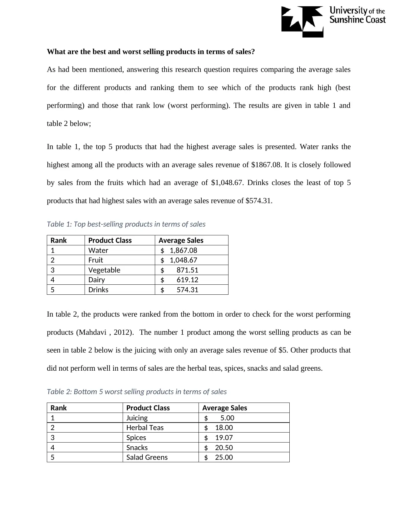
What are the best and worst selling products in terms of sales?
As had been mentioned, answering this research question requires comparing the average sales
for the different products and ranking them to see which of the products rank high (best
performing) and those that rank low (worst performing). The results are given in table 1 and
table 2 below;
In table 1, the top 5 products that had the highest average sales is presented. Water ranks the
highest among all the products with an average sales revenue of $1867.08. It is closely followed
by sales from the fruits which had an average of $1,048.67. Drinks closes the least of top 5
products that had highest sales with an average sales revenue of $574.31.
Table 1: Top best-selling products in terms of sales
Rank Product Class Average Sales
1 Water $ 1,867.08
2 Fruit $ 1,048.67
3 Vegetable $ 871.51
4 Dairy $ 619.12
5 Drinks $ 574.31
In table 2, the products were ranked from the bottom in order to check for the worst performing
products (Mahdavi , 2012). The number 1 product among the worst selling products as can be
seen in table 2 below is the juicing with only an average sales revenue of $5. Other products that
did not perform well in terms of sales are the herbal teas, spices, snacks and salad greens.
Table 2: Bottom 5 worst selling products in terms of sales
Rank Product Class Average Sales
1 Juicing $ 5.00
2 Herbal Teas $ 18.00
3 Spices $ 19.07
4 Snacks $ 20.50
5 Salad Greens $ 25.00
⊘ This is a preview!⊘
Do you want full access?
Subscribe today to unlock all pages.
Trusted by 1+ million students worldwide
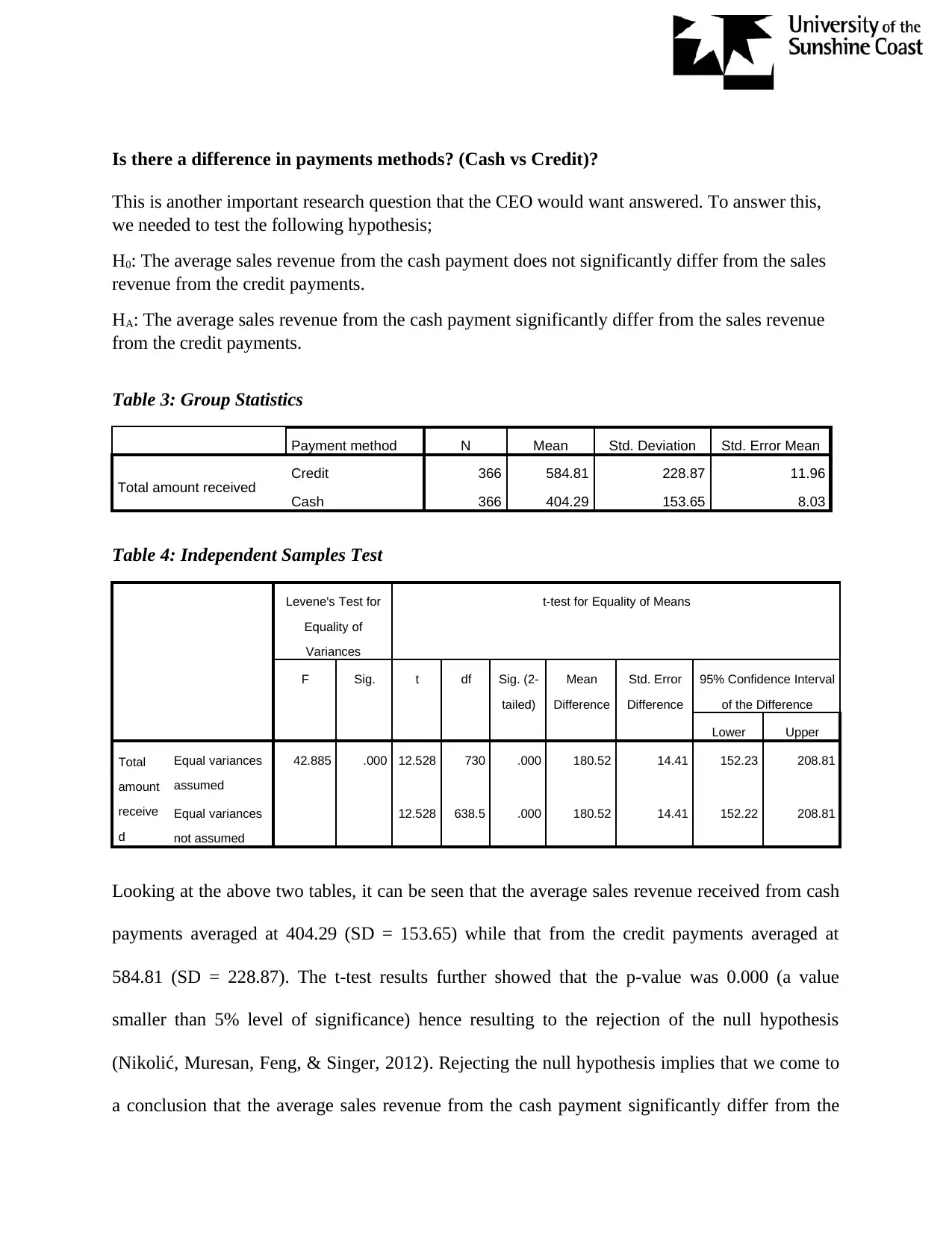
Is there a difference in payments methods? (Cash vs Credit)?
This is another important research question that the CEO would want answered. To answer this,
we needed to test the following hypothesis;
H0: The average sales revenue from the cash payment does not significantly differ from the sales
revenue from the credit payments.
HA: The average sales revenue from the cash payment significantly differ from the sales revenue
from the credit payments.
Table 3: Group Statistics
Payment method N Mean Std. Deviation Std. Error Mean
Total amount received Credit 366 584.81 228.87 11.96
Cash 366 404.29 153.65 8.03
Table 4: Independent Samples Test
Levene's Test for
Equality of
Variances
t-test for Equality of Means
F Sig. t df Sig. (2-
tailed)
Mean
Difference
Std. Error
Difference
95% Confidence Interval
of the Difference
Lower Upper
Total
amount
receive
d
Equal variances
assumed
42.885 .000 12.528 730 .000 180.52 14.41 152.23 208.81
Equal variances
not assumed
12.528 638.5 .000 180.52 14.41 152.22 208.81
Looking at the above two tables, it can be seen that the average sales revenue received from cash
payments averaged at 404.29 (SD = 153.65) while that from the credit payments averaged at
584.81 (SD = 228.87). The t-test results further showed that the p-value was 0.000 (a value
smaller than 5% level of significance) hence resulting to the rejection of the null hypothesis
(Nikolić, Muresan, Feng, & Singer, 2012). Rejecting the null hypothesis implies that we come to
a conclusion that the average sales revenue from the cash payment significantly differ from the
Paraphrase This Document
Need a fresh take? Get an instant paraphrase of this document with our AI Paraphraser
sales revenue from the credit payments. The amount received from the credit payments is by far
higher than what is received from the cash payments.
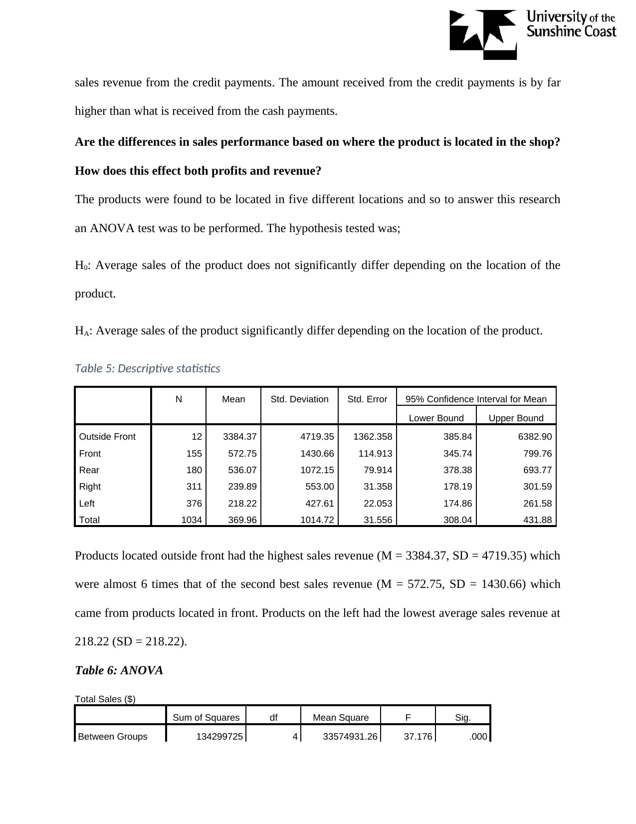
Are the differences in sales performance based on where the product is located in the shop?
How does this effect both profits and revenue?
The products were found to be located in five different locations and so to answer this research
an ANOVA test was to be performed. The hypothesis tested was;
H0: Average sales of the product does not significantly differ depending on the location of the
product.
HA: Average sales of the product significantly differ depending on the location of the product.
Table 5: Descriptive statistics
N Mean Std. Deviation Std. Error 95% Confidence Interval for Mean
Lower Bound Upper Bound
Outside Front 12 3384.37 4719.35 1362.358 385.84 6382.90
Front 155 572.75 1430.66 114.913 345.74 799.76
Rear 180 536.07 1072.15 79.914 378.38 693.77
Right 311 239.89 553.00 31.358 178.19 301.59
Left 376 218.22 427.61 22.053 174.86 261.58
Total 1034 369.96 1014.72 31.556 308.04 431.88
Products located outside front had the highest sales revenue (M = 3384.37, SD = 4719.35) which
were almost 6 times that of the second best sales revenue (M = 572.75, SD = 1430.66) which
came from products located in front. Products on the left had the lowest average sales revenue at
218.22 (SD = 218.22).
Table 6: ANOVA
Total Sales ($)
Sum of Squares df Mean Square F Sig.
Between Groups 134299725 4 33574931.26 37.176 .000
higher than what is received from the cash payments.
Are the differences in sales performance based on where the product is located in the shop?
How does this effect both profits and revenue?
The products were found to be located in five different locations and so to answer this research
an ANOVA test was to be performed. The hypothesis tested was;
H0: Average sales of the product does not significantly differ depending on the location of the
product.
HA: Average sales of the product significantly differ depending on the location of the product.
Table 5: Descriptive statistics
N Mean Std. Deviation Std. Error 95% Confidence Interval for Mean
Lower Bound Upper Bound
Outside Front 12 3384.37 4719.35 1362.358 385.84 6382.90
Front 155 572.75 1430.66 114.913 345.74 799.76
Rear 180 536.07 1072.15 79.914 378.38 693.77
Right 311 239.89 553.00 31.358 178.19 301.59
Left 376 218.22 427.61 22.053 174.86 261.58
Total 1034 369.96 1014.72 31.556 308.04 431.88
Products located outside front had the highest sales revenue (M = 3384.37, SD = 4719.35) which
were almost 6 times that of the second best sales revenue (M = 572.75, SD = 1430.66) which
came from products located in front. Products on the left had the lowest average sales revenue at
218.22 (SD = 218.22).
Table 6: ANOVA
Total Sales ($)
Sum of Squares df Mean Square F Sig.
Between Groups 134299725 4 33574931.26 37.176 .000
Within Groups 929333381 1029 903142.26
Total 1063633106 1033
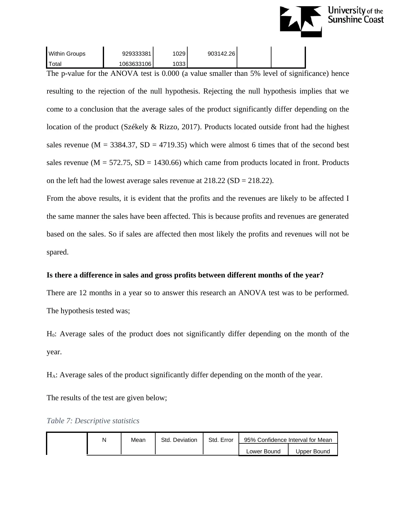
The p-value for the ANOVA test is 0.000 (a value smaller than 5% level of significance) hence
resulting to the rejection of the null hypothesis. Rejecting the null hypothesis implies that we
come to a conclusion that the average sales of the product significantly differ depending on the
location of the product (Székely & Rizzo, 2017). Products located outside front had the highest
sales revenue (M = 3384.37, SD = 4719.35) which were almost 6 times that of the second best
sales revenue (M = 572.75, SD = 1430.66) which came from products located in front. Products
on the left had the lowest average sales revenue at 218.22 (SD = 218.22).
From the above results, it is evident that the profits and the revenues are likely to be affected I
the same manner the sales have been affected. This is because profits and revenues are generated
based on the sales. So if sales are affected then most likely the profits and revenues will not be
spared.
Is there a difference in sales and gross profits between different months of the year?
There are 12 months in a year so to answer this research an ANOVA test was to be performed.
The hypothesis tested was;
H0: Average sales of the product does not significantly differ depending on the month of the
year.
HA: Average sales of the product significantly differ depending on the month of the year.
The results of the test are given below;
Table 7: Descriptive statistics
N Mean Std. Deviation Std. Error 95% Confidence Interval for Mean
Lower Bound Upper Bound
Total 1063633106 1033
The p-value for the ANOVA test is 0.000 (a value smaller than 5% level of significance) hence
resulting to the rejection of the null hypothesis. Rejecting the null hypothesis implies that we
come to a conclusion that the average sales of the product significantly differ depending on the
location of the product (Székely & Rizzo, 2017). Products located outside front had the highest
sales revenue (M = 3384.37, SD = 4719.35) which were almost 6 times that of the second best
sales revenue (M = 572.75, SD = 1430.66) which came from products located in front. Products
on the left had the lowest average sales revenue at 218.22 (SD = 218.22).
From the above results, it is evident that the profits and the revenues are likely to be affected I
the same manner the sales have been affected. This is because profits and revenues are generated
based on the sales. So if sales are affected then most likely the profits and revenues will not be
spared.
Is there a difference in sales and gross profits between different months of the year?
There are 12 months in a year so to answer this research an ANOVA test was to be performed.
The hypothesis tested was;
H0: Average sales of the product does not significantly differ depending on the month of the
year.
HA: Average sales of the product significantly differ depending on the month of the year.
The results of the test are given below;
Table 7: Descriptive statistics
N Mean Std. Deviation Std. Error 95% Confidence Interval for Mean
Lower Bound Upper Bound
⊘ This is a preview!⊘
Do you want full access?
Subscribe today to unlock all pages.
Trusted by 1+ million students worldwide
January 31 979.65 368.350 66.158 844.54 1114.76
February 29 1066.47 237.830 44.164 976.00 1156.94
March 31 1063.69 379.880 68.228 924.35 1203.03
April 30 1078.77 314.570 57.432 961.31 1196.23
May 31 1054.09 336.527 60.442 930.65 1177.53
June 30 918.81 223.442 40.795 835.38 1002.25
July 31 1004.78 248.080 44.556 913.79 1095.78
August 31 1025.26 308.806 55.463 911.99 1138.54
September 30 1014.06 302.101 55.156 901.25 1126.86
October 31 1056.03 353.343 63.462 926.42 1185.64
November 30 1197.64 343.489 62.712 1069.38 1325.90
December 31 1082.74 413.527 74.272 931.05 1234.42
Total 366 1044.97 326.285 17.055 1011.43 1078.51
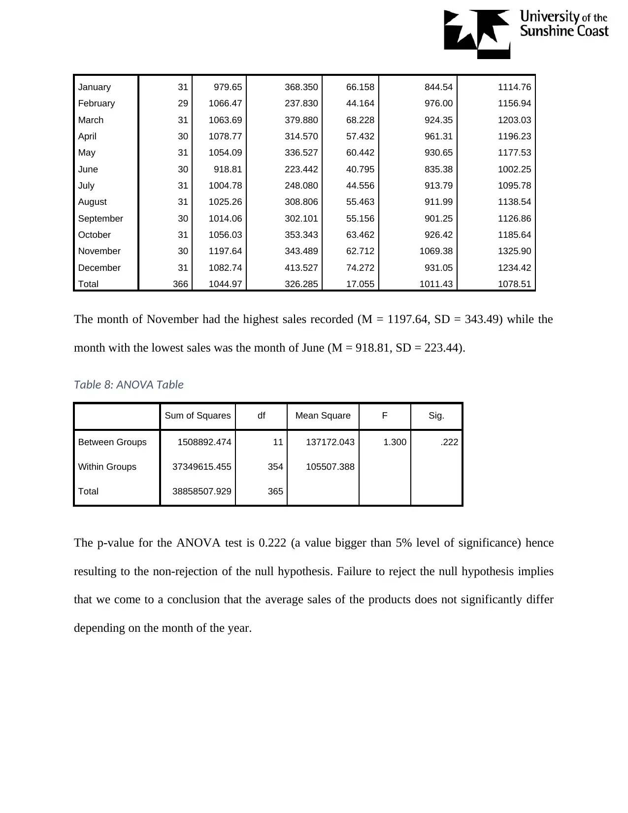
The month of November had the highest sales recorded (M = 1197.64, SD = 343.49) while the
month with the lowest sales was the month of June (M = 918.81, SD = 223.44).
Table 8: ANOVA Table
Sum of Squares df Mean Square F Sig.
Between Groups 1508892.474 11 137172.043 1.300 .222
Within Groups 37349615.455 354 105507.388
Total 38858507.929 365
The p-value for the ANOVA test is 0.222 (a value bigger than 5% level of significance) hence
resulting to the non-rejection of the null hypothesis. Failure to reject the null hypothesis implies
that we come to a conclusion that the average sales of the products does not significantly differ
depending on the month of the year.
February 29 1066.47 237.830 44.164 976.00 1156.94
March 31 1063.69 379.880 68.228 924.35 1203.03
April 30 1078.77 314.570 57.432 961.31 1196.23
May 31 1054.09 336.527 60.442 930.65 1177.53
June 30 918.81 223.442 40.795 835.38 1002.25
July 31 1004.78 248.080 44.556 913.79 1095.78
August 31 1025.26 308.806 55.463 911.99 1138.54
September 30 1014.06 302.101 55.156 901.25 1126.86
October 31 1056.03 353.343 63.462 926.42 1185.64
November 30 1197.64 343.489 62.712 1069.38 1325.90
December 31 1082.74 413.527 74.272 931.05 1234.42
Total 366 1044.97 326.285 17.055 1011.43 1078.51
The month of November had the highest sales recorded (M = 1197.64, SD = 343.49) while the
month with the lowest sales was the month of June (M = 918.81, SD = 223.44).
Table 8: ANOVA Table
Sum of Squares df Mean Square F Sig.
Between Groups 1508892.474 11 137172.043 1.300 .222
Within Groups 37349615.455 354 105507.388
Total 38858507.929 365
The p-value for the ANOVA test is 0.222 (a value bigger than 5% level of significance) hence
resulting to the non-rejection of the null hypothesis. Failure to reject the null hypothesis implies
that we come to a conclusion that the average sales of the products does not significantly differ
depending on the month of the year.
Paraphrase This Document
Need a fresh take? Get an instant paraphrase of this document with our AI Paraphraser
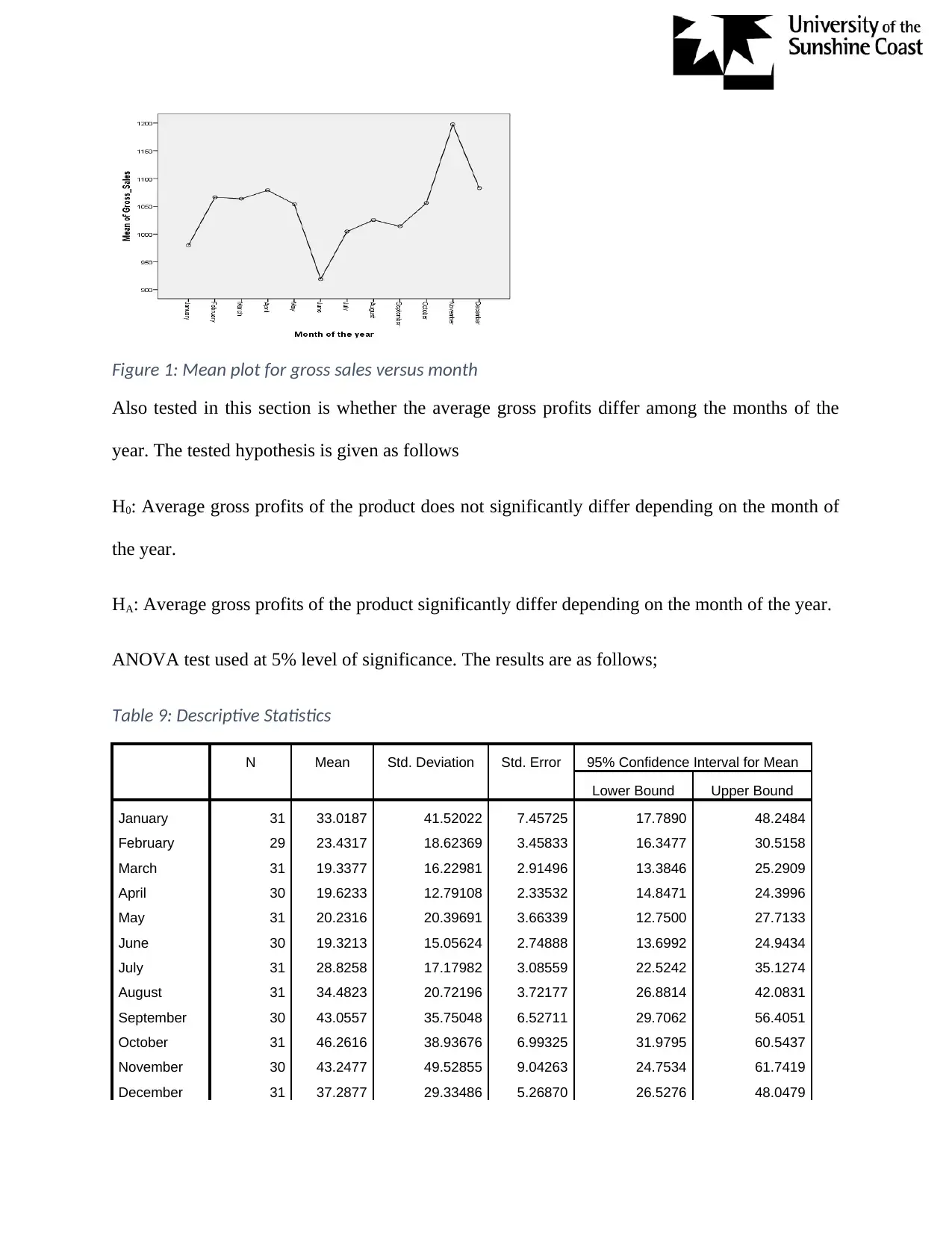
Figure 1: Mean plot for gross sales versus month
Also tested in this section is whether the average gross profits differ among the months of the
year. The tested hypothesis is given as follows
H0: Average gross profits of the product does not significantly differ depending on the month of
the year.
HA: Average gross profits of the product significantly differ depending on the month of the year.
ANOVA test used at 5% level of significance. The results are as follows;
Table 9: Descriptive Statistics
N Mean Std. Deviation Std. Error 95% Confidence Interval for Mean
Lower Bound Upper Bound
January 31 33.0187 41.52022 7.45725 17.7890 48.2484
February 29 23.4317 18.62369 3.45833 16.3477 30.5158
March 31 19.3377 16.22981 2.91496 13.3846 25.2909
April 30 19.6233 12.79108 2.33532 14.8471 24.3996
May 31 20.2316 20.39691 3.66339 12.7500 27.7133
June 30 19.3213 15.05624 2.74888 13.6992 24.9434
July 31 28.8258 17.17982 3.08559 22.5242 35.1274
August 31 34.4823 20.72196 3.72177 26.8814 42.0831
September 30 43.0557 35.75048 6.52711 29.7062 56.4051
October 31 46.2616 38.93676 6.99325 31.9795 60.5437
November 30 43.2477 49.52855 9.04263 24.7534 61.7419
December 31 37.2877 29.33486 5.26870 26.5276 48.0479
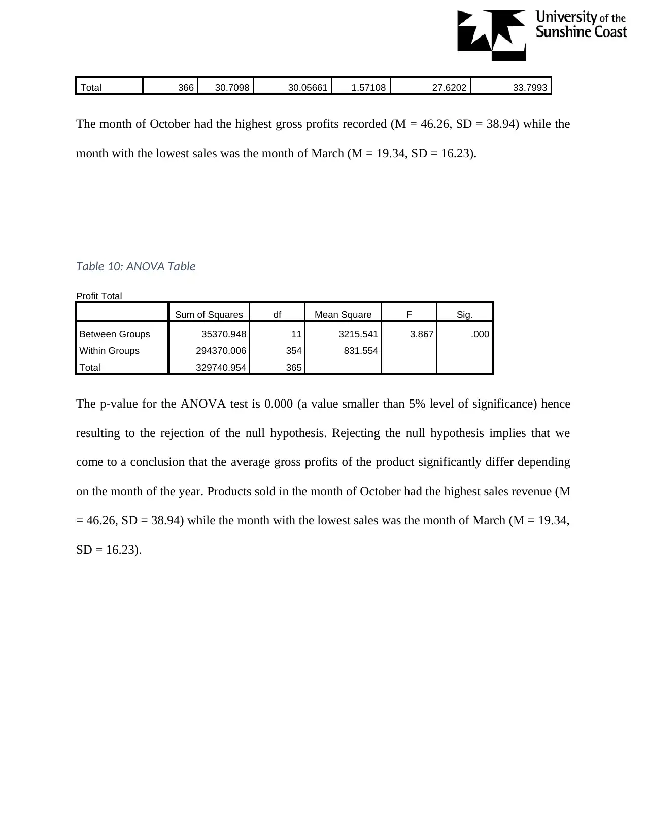
Total 366 30.7098 30.05661 1.57108 27.6202 33.7993
The month of October had the highest gross profits recorded (M = 46.26, SD = 38.94) while the
month with the lowest sales was the month of March (M = 19.34, SD = 16.23).
Table 10: ANOVA Table
Profit Total
Sum of Squares df Mean Square F Sig.
Between Groups 35370.948 11 3215.541 3.867 .000
Within Groups 294370.006 354 831.554
Total 329740.954 365
The p-value for the ANOVA test is 0.000 (a value smaller than 5% level of significance) hence
resulting to the rejection of the null hypothesis. Rejecting the null hypothesis implies that we
come to a conclusion that the average gross profits of the product significantly differ depending
on the month of the year. Products sold in the month of October had the highest sales revenue (M
= 46.26, SD = 38.94) while the month with the lowest sales was the month of March (M = 19.34,
SD = 16.23).
⊘ This is a preview!⊘
Do you want full access?
Subscribe today to unlock all pages.
Trusted by 1+ million students worldwide
1 out of 27
Related Documents


Your All-in-One AI-Powered Toolkit for Academic Success.
+13062052269
info@desklib.com
Available 24*7 on WhatsApp / Email
![[object Object]](/_next/static/media/star-bottom.7253800d.svg)
Unlock your academic potential
Copyright © 2020–2026 A2Z Services. All Rights Reserved. Developed and managed by ZUCOL.