GB513: Business Analytics - Unit 3 Assignment on Hypothesis Testing
VerifiedAdded on 2022/10/11
|11
|1917
|298
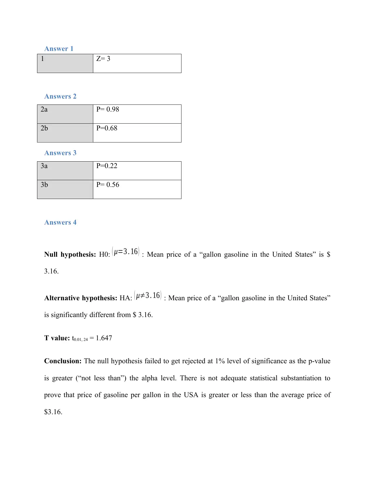
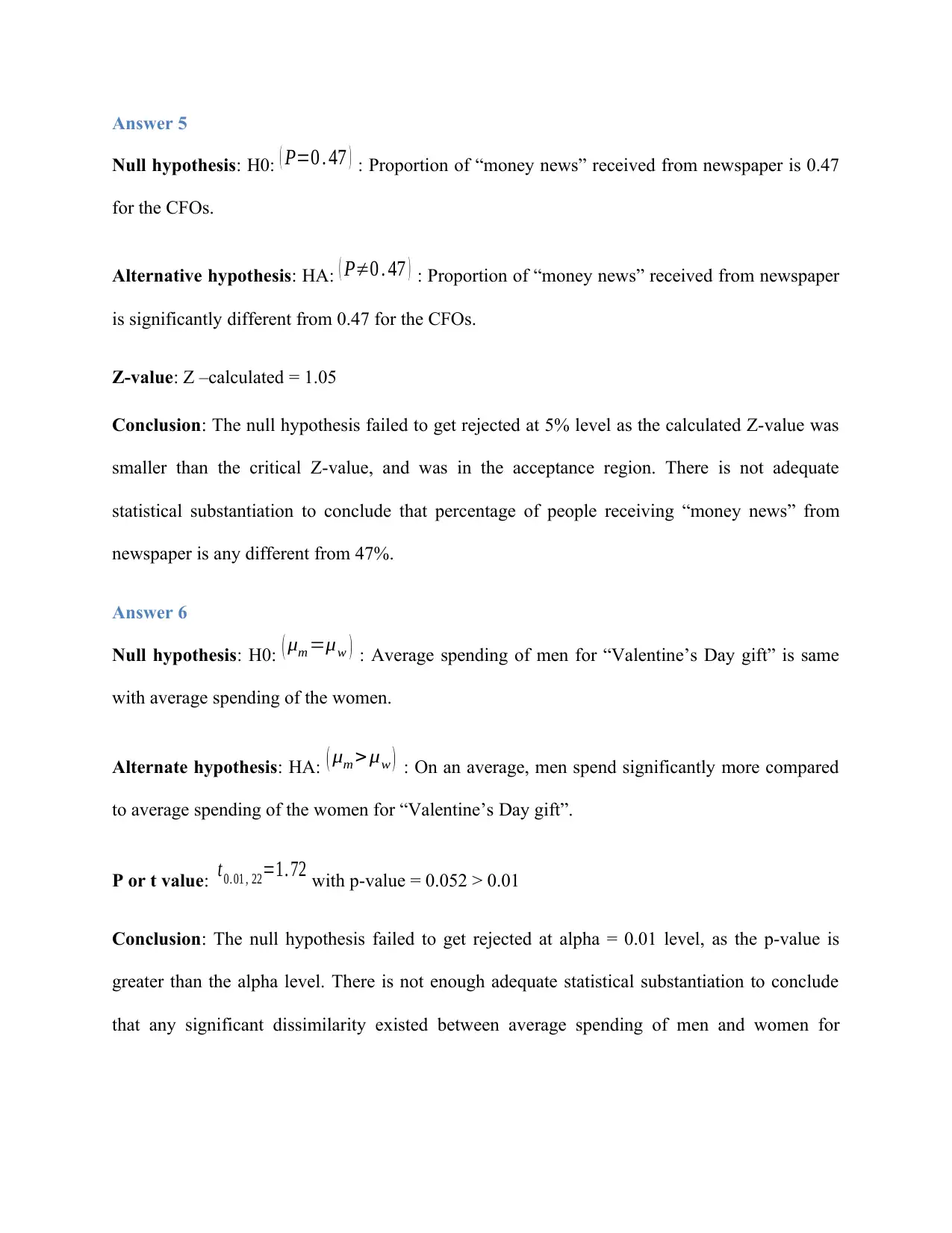
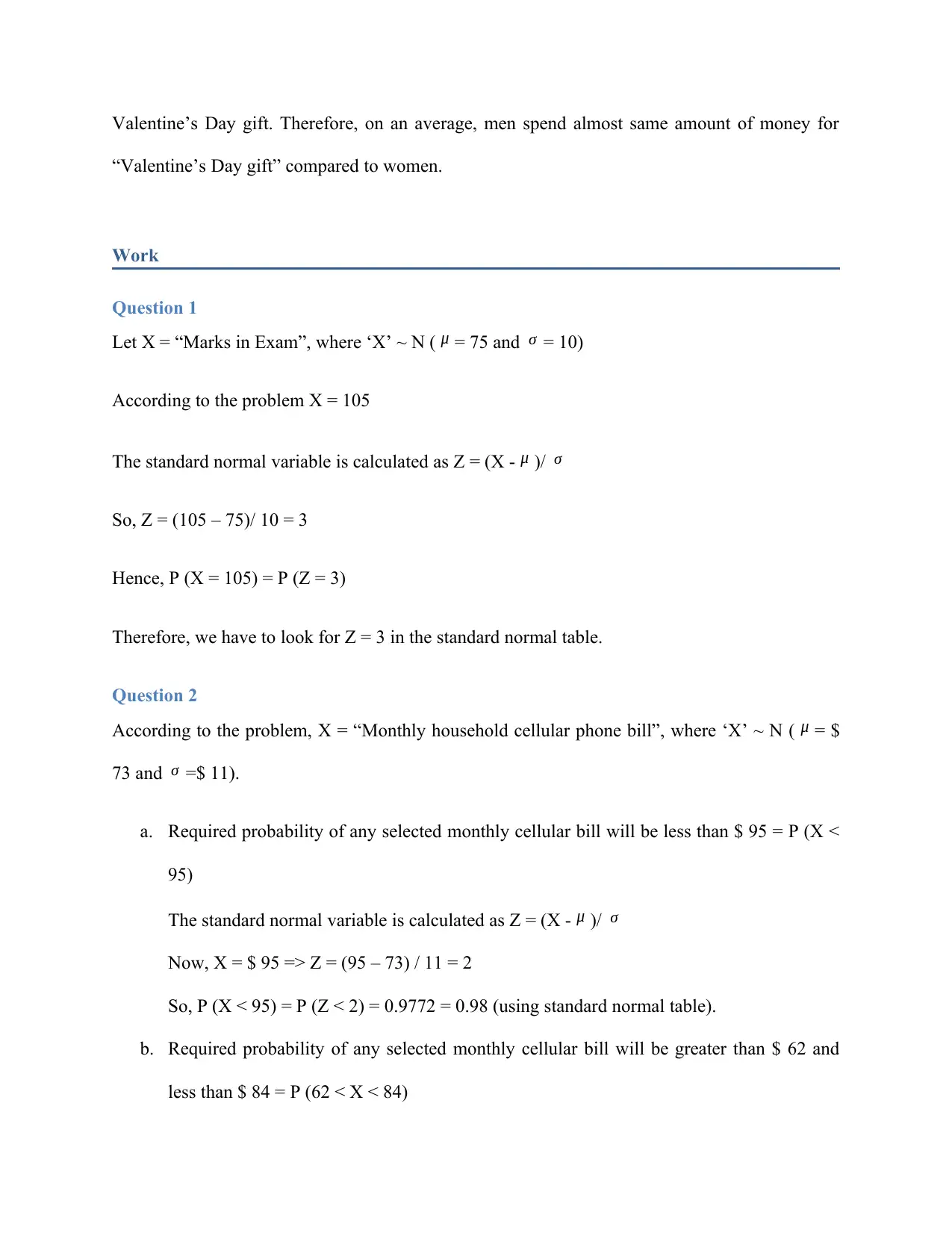
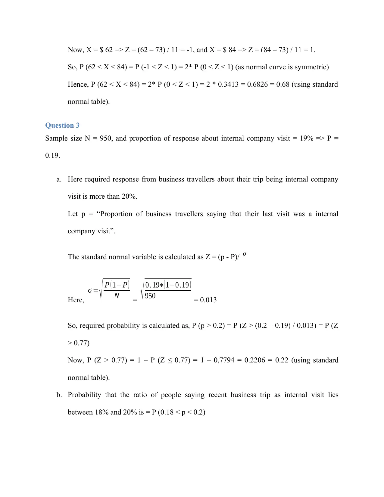
Homework Assignment
AI Summary
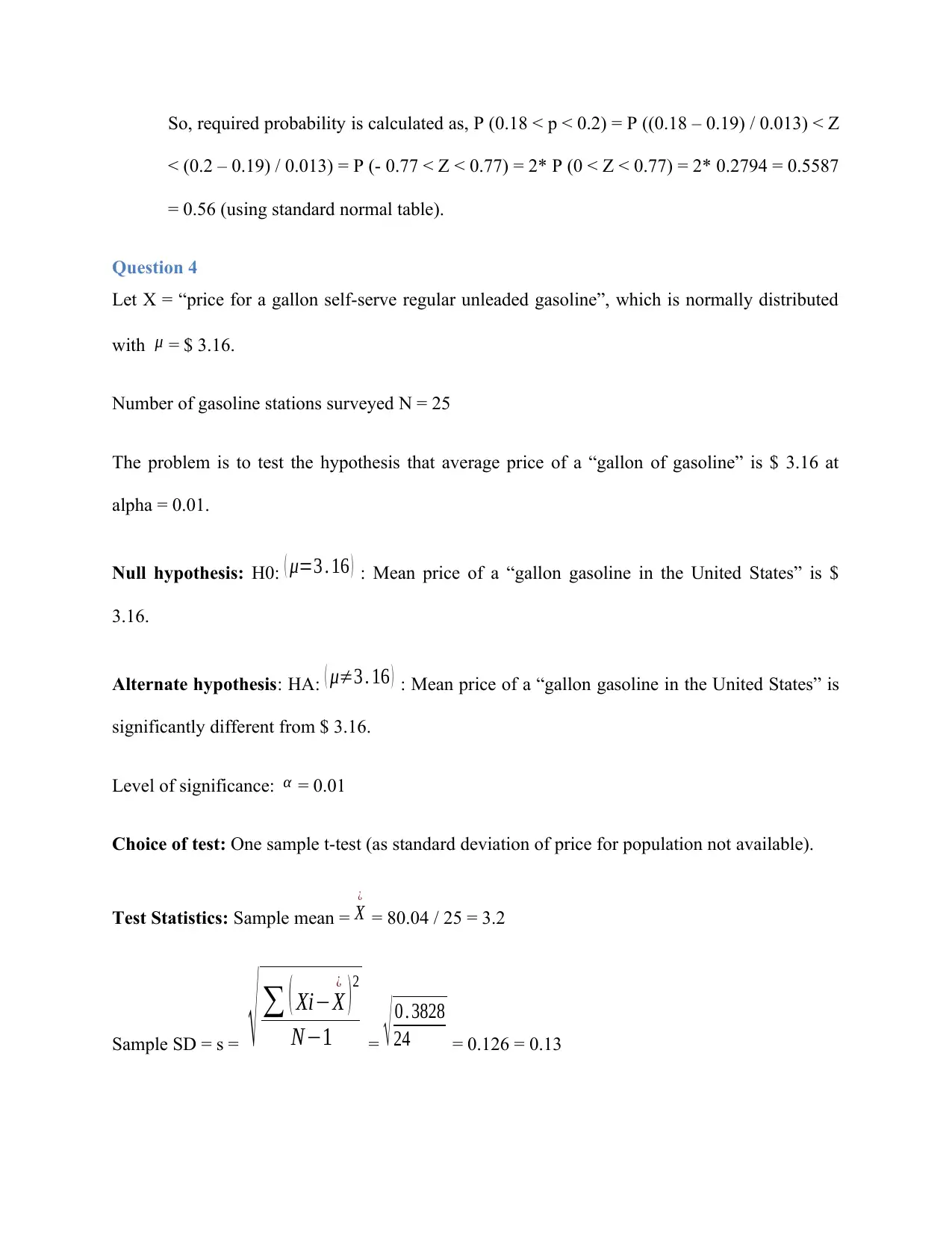
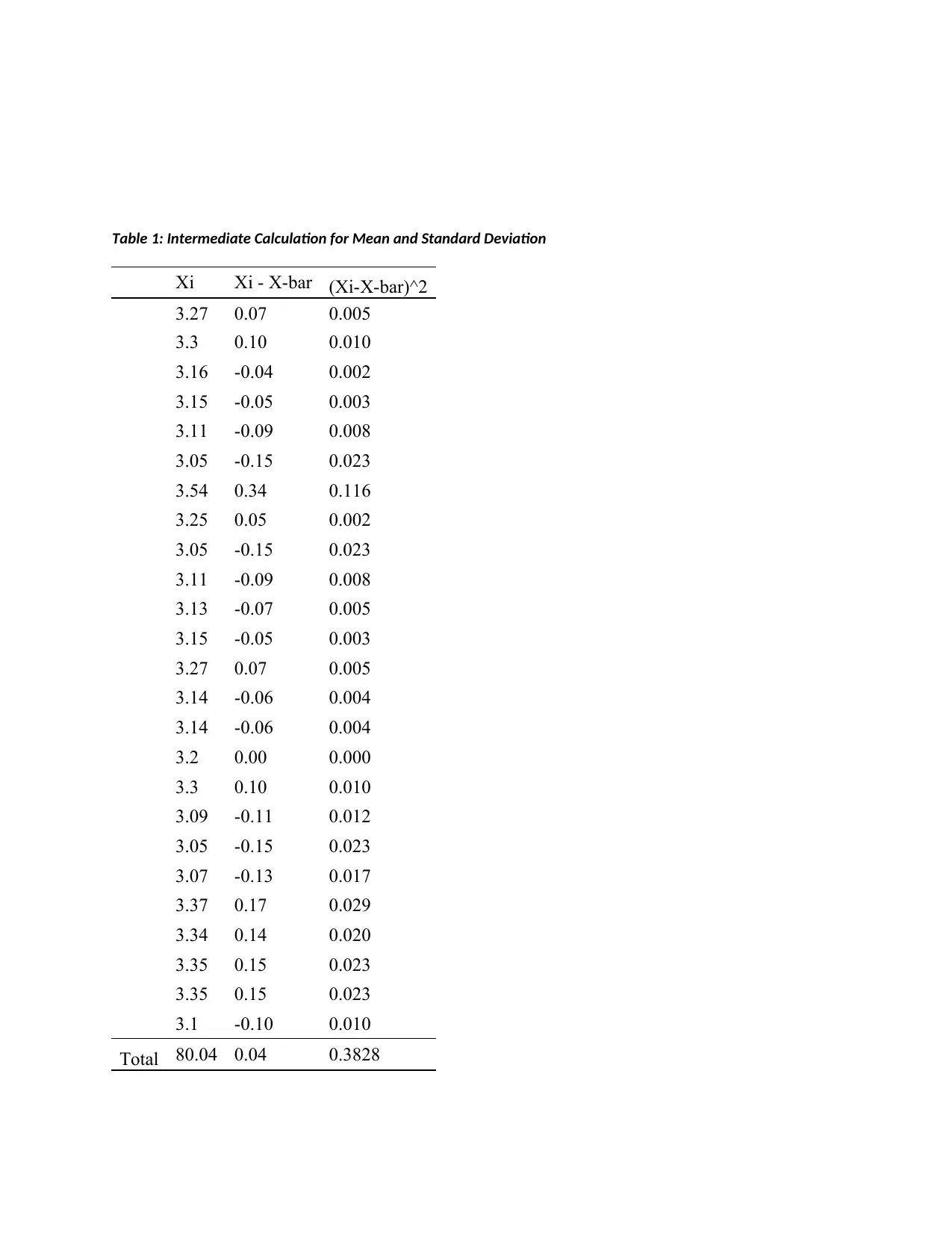
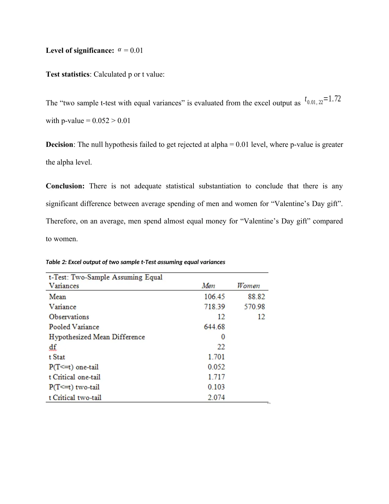
This document presents a comprehensive solution to a Business Analytics assignment, focusing on probability calculations and hypothesis testing. The solution includes detailed answers to questions involving z-values, t-tests, and the application of statistical concepts to real-world business scenarios. The assignment covers various aspects, including calculating probabilities based on normal distributions, hypothesis testing for population means and proportions, and the use of Excel for statistical analysis. The solution provides step-by-step calculations, null and alternative hypotheses, and conclusions based on p-values and significance levels. The assignment also involves interpreting the results of statistical tests and drawing meaningful conclusions about the data. The document provides a valuable resource for students studying business analytics, offering insights into the application of statistical methods in solving business problems.

1 out of 11


Your All-in-One AI-Powered Toolkit for Academic Success.
+13062052269
info@desklib.com
Available 24*7 on WhatsApp / Email
![[object Object]](/_next/static/media/star-bottom.7253800d.svg)
Copyright © 2020–2026 A2Z Services. All Rights Reserved. Developed and managed by ZUCOL.