University Business Statistics and Data Analysis: Car Sales Report

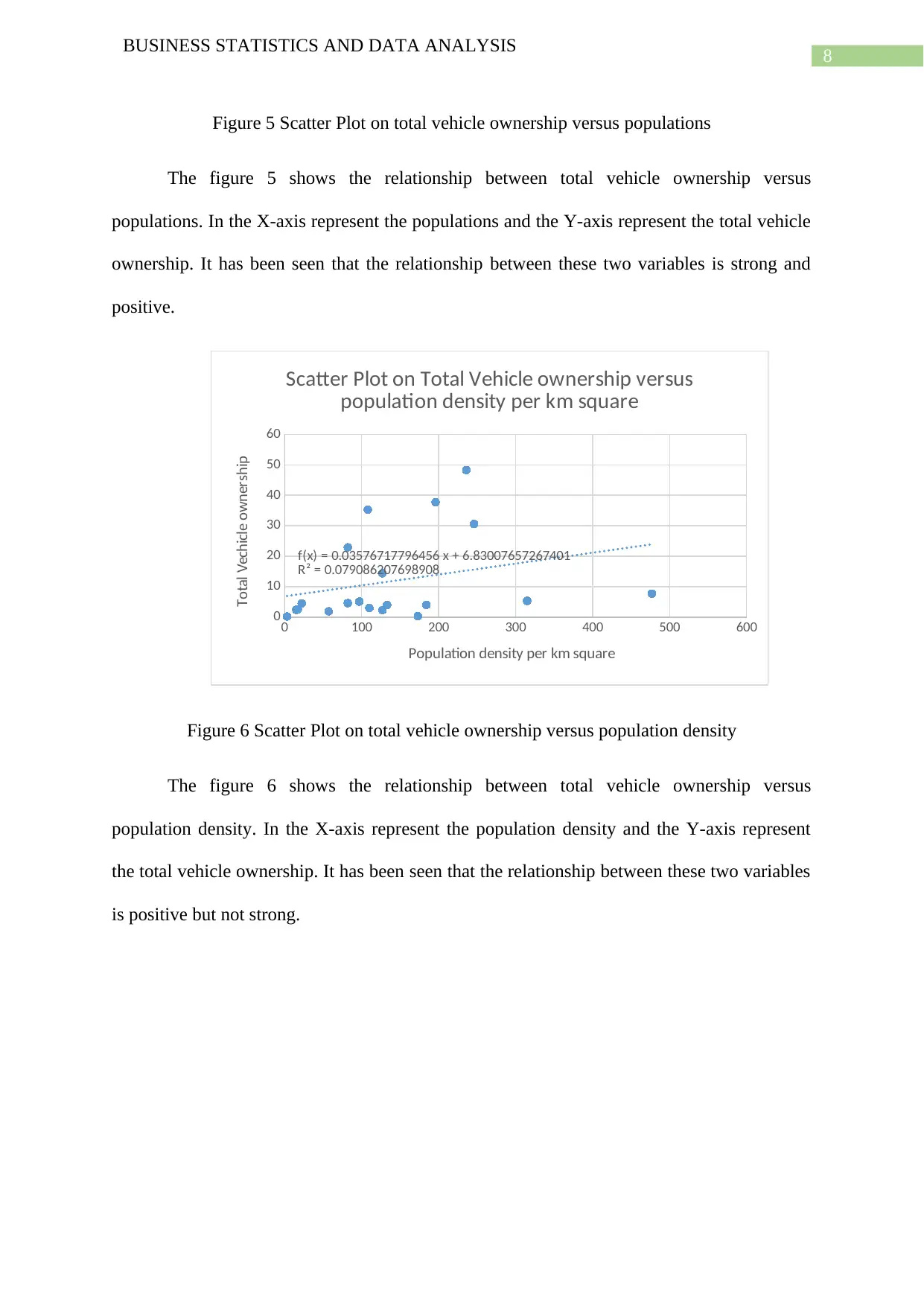
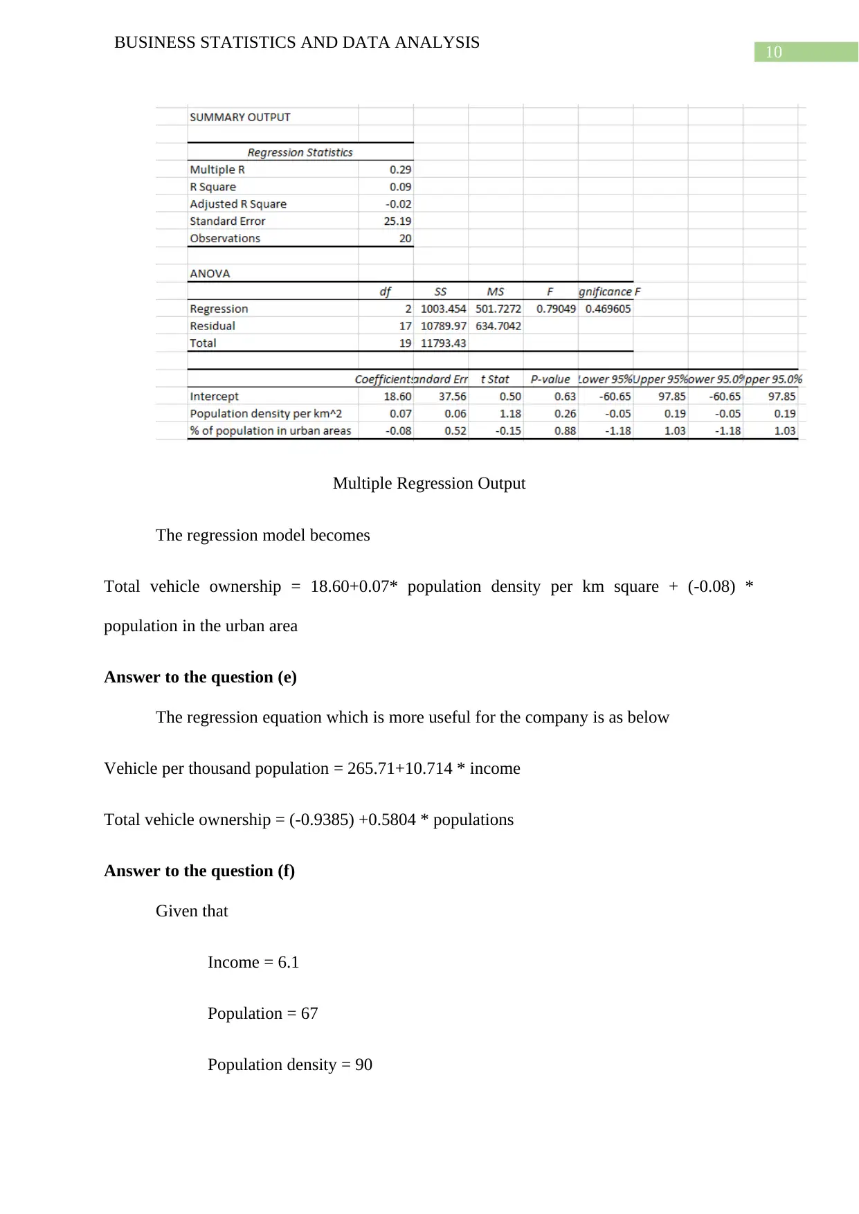
This report presents a data analysis and forecasting study of car sales distribution, focusing on vehicle ownership across different European countries. The analysis employs scatter plots and regression analysis to examine relationships between various variables, including vehicle ownership per 1000 population, income, population, population density, and urban population. The study investigates correlations between these variables and identifies key factors influencing car sales. Regression models are developed to forecast vehicle ownership, and the report concludes with a discussion of the findings, comparing predicted and actual values, and offering insights for AutoMobile Inc.'s potential market expansion. The report includes scatter plots illustrating the relationships between different variables and provides multiple regression outputs. The conclusion summarizes the key findings, highlighting the relationships between variables like income and total vehicle ownership, and offers insights into the accuracy of the predictions.

Running head: BUSINESS STATISTICS AND DATA ANALYSIS
Business Statistics and Data Analysis
Name of the student:
Name of the University:
Author note:

1
BUSINESS STATISTICS AND DATA ANALYSIS
Abstract
The study is based on data analysis and forecasting of car sales distribution. The aim of the
study is to test the vehicle ownership among different European countries. The study shows
the relationship of car sales among different area with the help of scatter plot and regression
analysis.

2
BUSINESS STATISTICS AND DATA ANALYSIS
Table of Contents
Abstract......................................................................................................................................1
Introduction................................................................................................................................3
Discussion..................................................................................................................................4
Answer to the question (a).....................................................................................................4
Answer to the question (b).....................................................................................................6
Answer to the question (c).....................................................................................................7
Answer to the question (d).....................................................................................................9
Answer to the question (e)...................................................................................................10
Answer to the question (f)....................................................................................................10
Conclusion................................................................................................................................12
References and Bibliography...................................................................................................13
Appendices...............................................................................................................................14

3
BUSINESS STATISTICS AND DATA ANALYSIS
Introduction
The study is based on data analysis and forecasting of car sales distribution. . The aim
of the study is to test the vehicle ownership among different European countries (Barreira,
Godinho and Melo 2013). The study shows the relationship of car sales among different area
with the help of scatter plot and regression analysis. The different variable of the study is
vehicle per thousand population, income, population, population density, population in urban
area and total vehicles ownership. The dependent variables of the study are vehicle per
thousand population and total vehicles ownership (Chatterjee and Hadi 2015). Similarly the
independent variables are population, population density, population in urban area. There are
various scatter plot has been drawn with respect to different independent variable. Among the
scatter plot the best and close to the dependent variable plot are selected. Moreover a multiple
linear regression model has been presented. With the help of some specific value the
dependent variable of the study is forecasted.

4
BUSINESS STATISTICS AND DATA ANALYSIS
Discussion
Answer to the question (a)
5 10 15 20 25 30 35 40 45
0
100
200
300
400
500
600
700
800
f(x) = 10.7140607093045 x + 265.705307867506
R² = 0.524276234325444
Scatter Plot on vehicles per 1000 populationsversus
Income
Income
Vechicles per 1000 populations
Figure 1 Scatter Plot on vehicles per 1000 population versus income
The figure 1 shows the relationship between vehicles per 1000 population versus
income. In the X-axis represent the income and the Y-axis represent the vehicles per 1000
population. It has been seen that the relationship between these two variable is positive and
strong.
0 10 20 30 40 50 60 70 80 90
0
100
200
300
400
500
600
700
800
f(x) = 0.684625938409498 x + 503.364267447147
R² = 0.0261604503904173
Scatter Plot on Vehicles per 1000 populations
versus population
Populations
Vechicles per 1000 populations
Figure 2 Scatter Plot on vehicles per 1000 population versus populations

5
BUSINESS STATISTICS AND DATA ANALYSIS
The figure 2 shows the relationship between vehicles per 1000 population versus
populations. In the X-axis represent the population and the Y-axis represent the vehicles per
1000 population. It has been seen that the relationship between these two variable is positive
and but not strong.
0 100 200 300 400 500 600
0
100
200
300
400
500
600
700
800
f(x) = 0.0141247886400172 x + 516.467585914374
R² = 0.000237964518570166
Scatter Plot on Vehicles per 1000 populations
versus population density
Population density
Vechicles per 1000 popualtions
Figure 3 Scatter Plot on vehicles per 1000 population versus population density
The figure 3 shows the relationship between vehicles per 1000 population versus
population density. In the X-axis represent the population density and the Y-axis represent
the vehicles per 1000 population. It has been seen that the relationship between these two
variable is positive and but not strong.

6
BUSINESS STATISTICS AND DATA ANALYSIS
55 60 65 70 75 80 85 90 95 100
0
100
200
300
400
500
600
700
800
f(x) = 3.32491146826478 x + 263.761781530918
R² = 0.153650187199907
Scatter Plot on Vechicles Per 1000 populations
versus population in Urban Areas
Population in Urban area
Vechicles per 1000 populations
Figure 4 Scatter Plot on vehicles per 1000 population versus population in urban area
The figure 4 shows the relationship between vehicles per 1000 population versus
population in urban area. In the X-axis represent the population in urban area and the Y-axis
represent the vehicles per 1000 population. It has been seen that the relationship between
these two variable is positive and but not strong.
Answer to the question (b)
Among all the scatter plot it has been seen that only the variable vehicles per 1000
population versus income shows positive and strong relation. Thus this means that the
variable population is closely correlated to the vehicles per thousand population.

7
BUSINESS STATISTICS AND DATA ANALYSIS
Multiple Regression Output
The regression model becomes
Vehicles per 1000 population = 151.32+11.68*income+1.73*population+ (-1.19) *
population density per km square +1.04 * population in urban populations.
Answer to the question (c)
0 10 20 30 40 50 60 70 80 90
0
10
20
30
40
50
60
f(x) = 0.580372937447224 x − 0.938517676649585
R² = 0.974396989311985
Scatter Plot on Total Vehicle ownership versus
populations
Populations
Total Vechicle Ownership

8
BUSINESS STATISTICS AND DATA ANALYSIS
Figure 5 Scatter Plot on total vehicle ownership versus populations
The figure 5 shows the relationship between total vehicle ownership versus
populations. In the X-axis represent the populations and the Y-axis represent the total vehicle
ownership. It has been seen that the relationship between these two variables is strong and
positive.
0 100 200 300 400 500 600
0
10
20
30
40
50
60
f(x) = 0.03576717796456 x + 6.83007657267401
R² = 0.079086207698908
Scatter Plot on Total Vehicle ownership versus
population density per km square
Population density per km square
Total Vechicle ownership
Figure 6 Scatter Plot on total vehicle ownership versus population density
The figure 6 shows the relationship between total vehicle ownership versus
population density. In the X-axis represent the population density and the Y-axis represent
the total vehicle ownership. It has been seen that the relationship between these two variables
is positive but not strong.

9
BUSINESS STATISTICS AND DATA ANALYSIS
55 60 65 70 75 80 85 90 95 100
0
10
20
30
40
50
60
f(x) = 0.138415962952874 x + 1.24733723780986
R² = 0.0138015666591467
Scatter Plot on Total Vehicle ownership versus
Population in Urban area
Urban Population
Total vechicle ownership
Figure 7 Scatter Plot on total vehicle ownership versus urban population
The figure 7 shows the relationship between total vehicle ownership versus urban
population. In the X-axis represent the urban population and the Y-axis represent the total
vehicle ownership. It has been seen that the relationship between these two variables is
positive but not strong.
Answer to the question (d)
Among all the scatter plot it has been seen that only the variable total vehicle
ownership versus populations shows positive and strong relation. Thus this means that the
variable population is closely correlated to the total vehicle ownership.

10
BUSINESS STATISTICS AND DATA ANALYSIS
Multiple Regression Output
The regression model becomes
Total vehicle ownership = 18.60+0.07* population density per km square + (-0.08) *
population in the urban area
Answer to the question (e)
The regression equation which is more useful for the company is as below
Vehicle per thousand population = 265.71+10.714 * income
Total vehicle ownership = (-0.9385) +0.5804 * populations
Answer to the question (f)
Given that
Income = 6.1
Population = 67
Population density = 90

11
BUSINESS STATISTICS AND DATA ANALYSIS
% urban = 67
Hence
Vehicles per 1000 population = 151.32+11.68*income+1.73*population+ (-1.19) *
population density per km square +1.04 * population in urban populations.
= 151.32+11.68*6.1+1.73*67+ (-1.19) * 90+1.04 * 67
= 391.3235
Total vehicle ownership = 18.60+0.07* population density per km square + (-0.08) *
population in the urban area
= 18.60+0.07* 90+ (-0.08) * 67
= 19.425
The difference between the actual and predicted value is called the residual. The
reason of residual is that the prediction is very high as compared to real value. The main
reason of the difference is the estimated predicted value is very high as compared to the
actual.