NCI Business Data Analysis Exam: Hypothesis Testing & Regression

This document provides solutions to a Business Data Analysis exam covering topics such as hypothesis testing, ANOVA, and moving averages. The first question involves conducting a t-test to determine if there is a significant difference between the salaries of male and female professors. The second question uses a paired t-test to analyze blood glucose levels before and after a program for diabetic patients. The third question interprets a one-way ANOVA table and performs another ANOVA test to compare test scores from three different classes. The final question uses a chi-square test to analyze survey responses and applies simple and weighted moving averages to estimate future rates based on historical data from the Road Authority Of Ireland. Desklib is a platform where students can find past papers and solved assignments.

Business Analysis
Student Name
Course Name
Institution Affiliation

Business Analysis
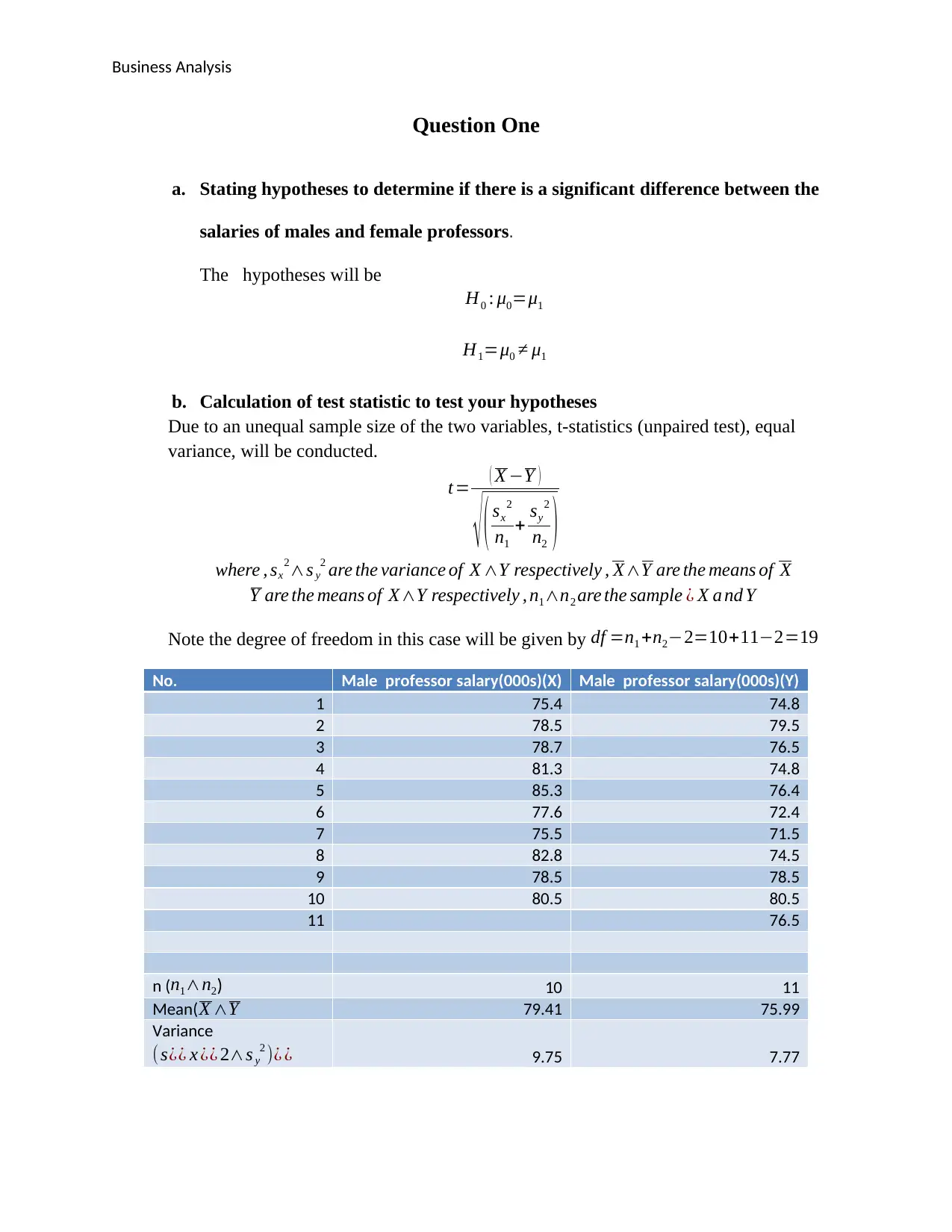
Question One
a. Stating hypotheses to determine if there is a significant difference between the
salaries of males and female professors.
The hypotheses will be
H0 : μ0=μ1
H1=μ0 ≠ μ1
b. Calculation of test statistic to test your hypotheses
Due to an unequal sample size of the two variables, t-statistics (unpaired test), equal
variance, will be conducted.
t= ( X −Y )
√ ( sx
2
n1
+ sy
2
n2 )
where , sx
2∧s y
2 are the variance of X ∧Y respectively , X∧Y are the means of X
Y are the means of X∧Y respectively , n1∧n2 are the sample ¿ X a nd Y
Note the degree of freedom in this case will be given by df =n1 +n2−2=10+11−2=19
No. Male professor salary(000s)(X) Male professor salary(000s)(Y)
1 75.4 74.8
2 78.5 79.5
3 78.7 76.5
4 81.3 74.8
5 85.3 76.4
6 77.6 72.4
7 75.5 71.5
8 82.8 74.5
9 78.5 78.5
10 80.5 80.5
11 76.5
n (n1∧n2) 10 11
Mean( X ∧Y 79.41 75.99
Variance
(s¿¿ x ¿¿ 2∧s y
2 )¿ ¿ 9.75 7.77

Business Analysis
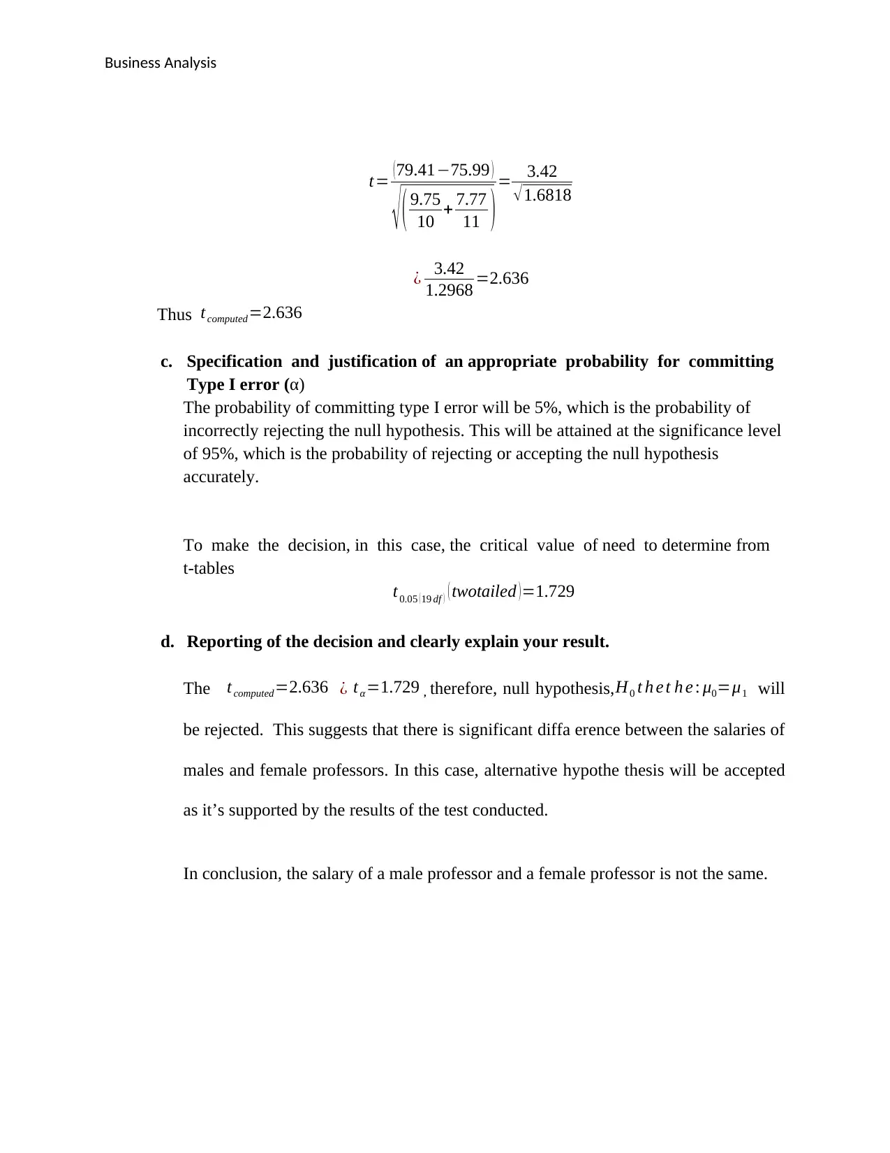
t= (79.41−75.99 )
√ ( 9.75
10 + 7.77
11 )= 3.42
√1.6818
¿ 3.42
1.2968 =2.636
Thus tcomputed=2.636
c. Specification and justification of an appropriate probability for committing
Type I error (α)
The probability of committing type I error will be 5%, which is the probability of
incorrectly rejecting the null hypothesis. This will be attained at the significance level
of 95%, which is the probability of rejecting or accepting the null hypothesis
accurately.
To make the decision, in this case, the critical value of need to determine from
t-tables
t0.05 ( 19 df ) ( twotailed ) =1.729
d. Reporting of the decision and clearly explain your result.
The tcomputed=2.636 ¿ tα=1.729 , therefore, null hypothesis,H0 t h e t h e : μ0=μ1 will
be rejected. This suggests that there is significant diffa erence between the salaries of
males and female professors. In this case, alternative hypothe thesis will be accepted
as it’s supported by the results of the test conducted.
In conclusion, the salary of a male professor and a female professor is not the same.

Business Analysis
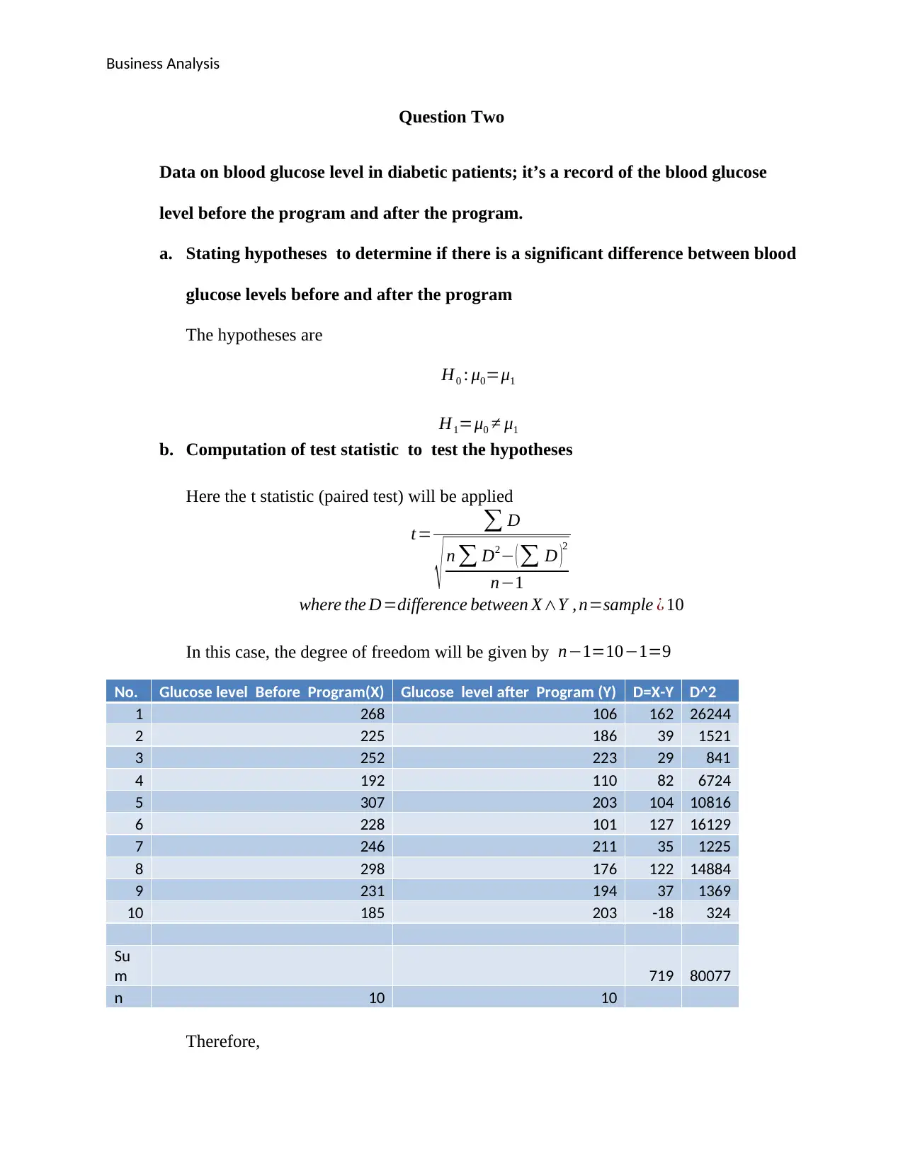
Question Two
Data on blood glucose level in diabetic patients; it’s a record of the blood glucose
level before the program and after the program.
a. Stating hypotheses to determine if there is a significant difference between blood
glucose levels before and after the program
The hypotheses are
H0 : μ0=μ1
H1=μ0 ≠ μ1
b. Computation of test statistic to test the hypotheses
Here the t statistic (paired test) will be applied
t= ∑ D
√ n ∑ D2− ( ∑ D )
2
n−1
where the D=difference between X∧Y , n=sample ¿ 10
In this case, the degree of freedom will be given by n−1=10−1=9
No. Glucose level Before Program(X) Glucose level after Program (Y) D=X-Y D^2
1 268 106 162 26244
2 225 186 39 1521
3 252 223 29 841
4 192 110 82 6724
5 307 203 104 10816
6 228 101 127 16129
7 246 211 35 1225
8 298 176 122 14884
9 231 194 37 1369
10 185 203 -18 324
Su
m 719 80077
n 10 10
Therefore,

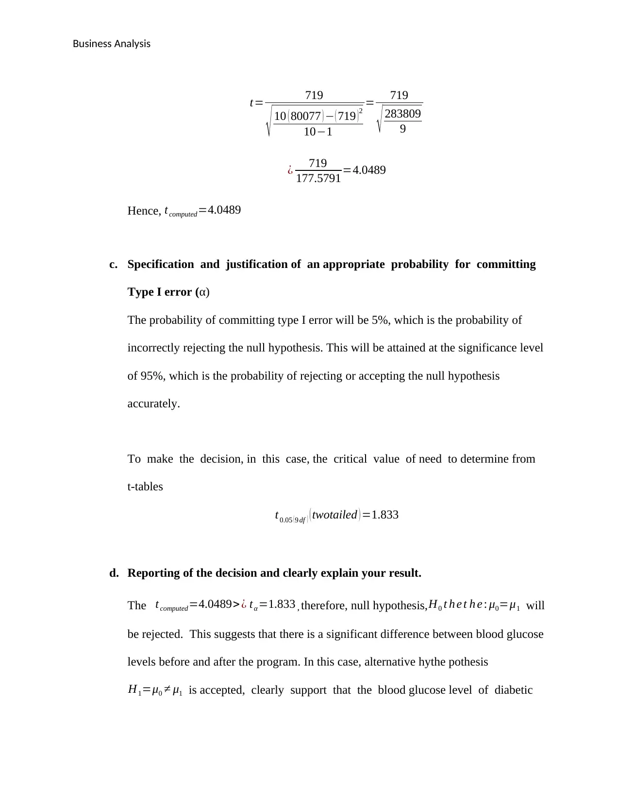
Business Analysis
t= 719
√ 10 ( 80077 ) − ( 719 )2
10−1
= 719
√ 283809
9
¿ 719
177.5791=4.0489
Hence, tcomputed=4.0489
c. Specification and justification of an appropriate probability for committing
Type I error (α)
The probability of committing type I error will be 5%, which is the probability of
incorrectly rejecting the null hypothesis. This will be attained at the significance level
of 95%, which is the probability of rejecting or accepting the null hypothesis
accurately.
To make the decision, in this case, the critical value of need to determine from
t-tables
t0.05 (9 df ) ( twotailed ) =1.833
d. Reporting of the decision and clearly explain your result.
The tcomputed=4.0489> ¿ tα =1.833 , therefore, null hypothesis, H0 t h e t h e : μ0=μ1 will
be rejected. This suggests that there is a significant difference between blood glucose
levels before and after the program. In this case, alternative hythe pothesis
H1=μ0 ≠ μ1 is accepted, clearly support that the blood glucose level of diabetic

Business Analysis
people cannot be the same, at any time, due to the difference in metabolic rate
in the body systems.
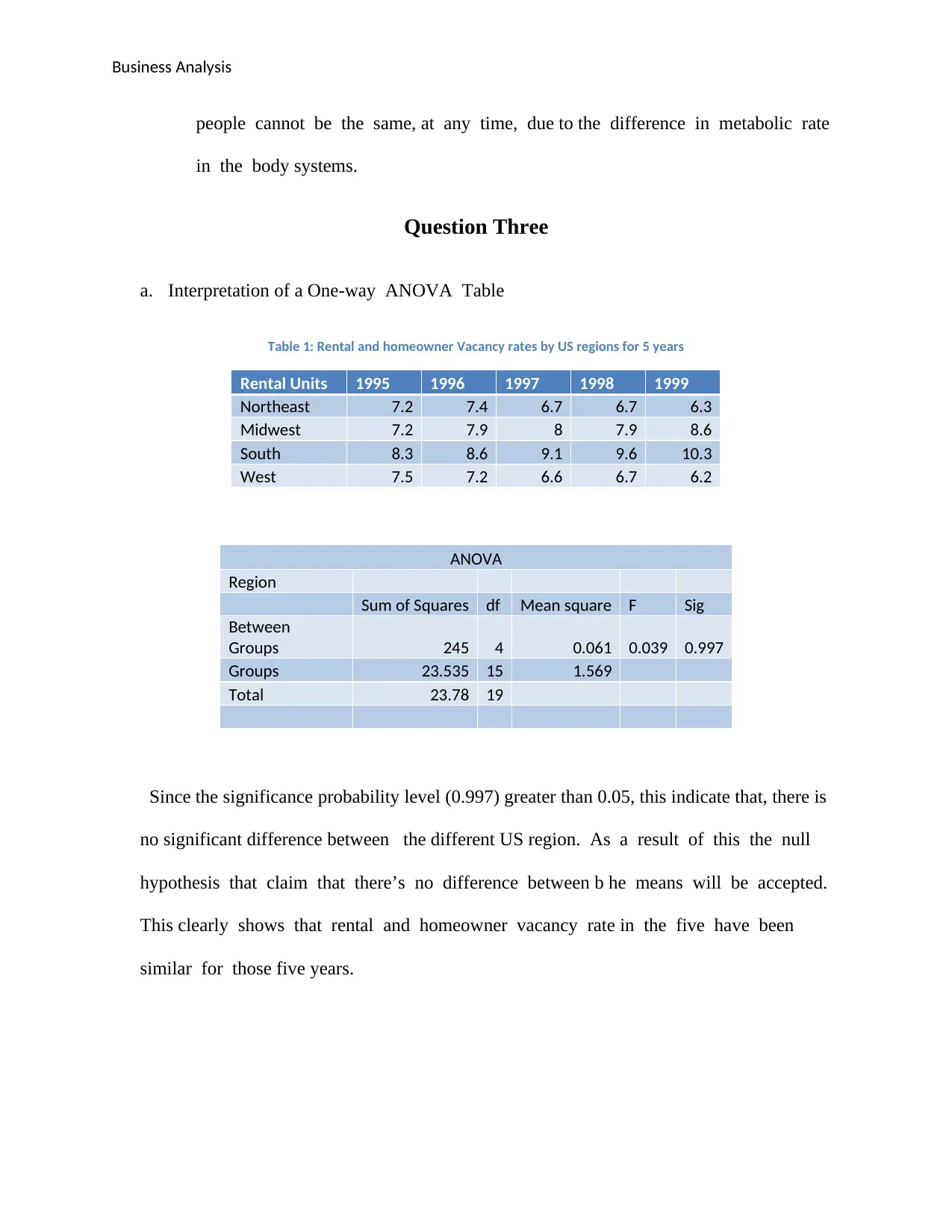
Question Three
a. Interpretation of a One-way ANOVA Table
Table 1: Rental and homeowner Vacancy rates by US regions for 5 years
Rental Units 1995 1996 1997 1998 1999
Northeast 7.2 7.4 6.7 6.7 6.3
Midwest 7.2 7.9 8 7.9 8.6
South 8.3 8.6 9.1 9.6 10.3
West 7.5 7.2 6.6 6.7 6.2
ANOVA
Region
Sum of Squares df Mean square F Sig
Between
Groups 245 4 0.061 0.039 0.997
Groups 23.535 15 1.569
Total 23.78 19
Since the significance probability level (0.997) greater than 0.05, this indicate that, there is
no significant difference between the different US region. As a result of this the null
hypothesis that claim that there’s no difference between b he means will be accepted.
This clearly shows that rental and homeowner vacancy rate in the five have been
similar for those five years.

Business Analysis
b. Data of test score from three classes
i. Stating the hypotheses to determine if there is a significant difference
between the different classes
The hypotheses will be,
H0 : μ0=μ1 =μ2
H0 : μ0 ≠ μ1∨μ0 ≠ μ2∨μ1=μ2
ii. Calculation of test statistic to test the hypotheses
For the case above, one-way ANOVA is required, where F-statistic will be determined,
because the sample has more than two groups, has three. This involves comparison of
the between the groups and within the groups.
F=
SSb
Df b
SSW
Df W
= Mean Squarebetween
Mean Squarewithin
Within-group Sum of Square ( SSW )
SSW =∑
j=1
p
∑
i=1
n
( Xi , j −X j ) 2
No. Class 1 Class 2 Class 3
X j d= X j −X j d^2 X j d= X j −X j d^2 X j d= X j −X j d^2
1 64 -12 144 56 -10.33 106.78 81 -4.67 21.78
2 84 8 64 74 7.67 58.78 92 6.33 40.11
3 75 -1 1 69 2.67 7.11 84 -1.67 2.78
4 77 1 1
5 80 4 16
n 5 3 3
Mean 76 66.33 85.67
Sum of Squares 226 172.67 64.67
where , Xi , j are theobservations ∈groups∧X j average of group J

Business Analysis
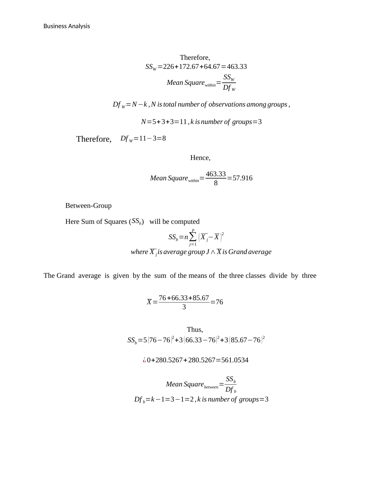
Therefore,
SSW =226+172.67+64.67=463.33
Mean Squarewithin= SSW
Df W
Df W =N −k , N is total number of observations among groups ,
N=5+ 3+3=11 , k is number of groups=3
Therefore, Df W =11−3=8
Hence,
Mean Squarewithin= 463.33
8 =57.916
Between-Group
Here Sum of Squares ( SSb) will be computed
SSb =n∑
j=1
p
( X j−X )2
where X j is average group J ∧ X is Grand average
The Grand average is given by the sum of the means of the three classes divide by three
X =76 +66.33+85.67
3 =76
Thus,
SSb =5 (76−76 )2 +3 ( 66.33−76 )2 +3 ( 85.67−76 )2
¿ 0+280.5267+ 280.5267=561.0534
Mean Squarebetween= SSb
Df b
Df b=k −1=3−1=2 , k is number of groups=3

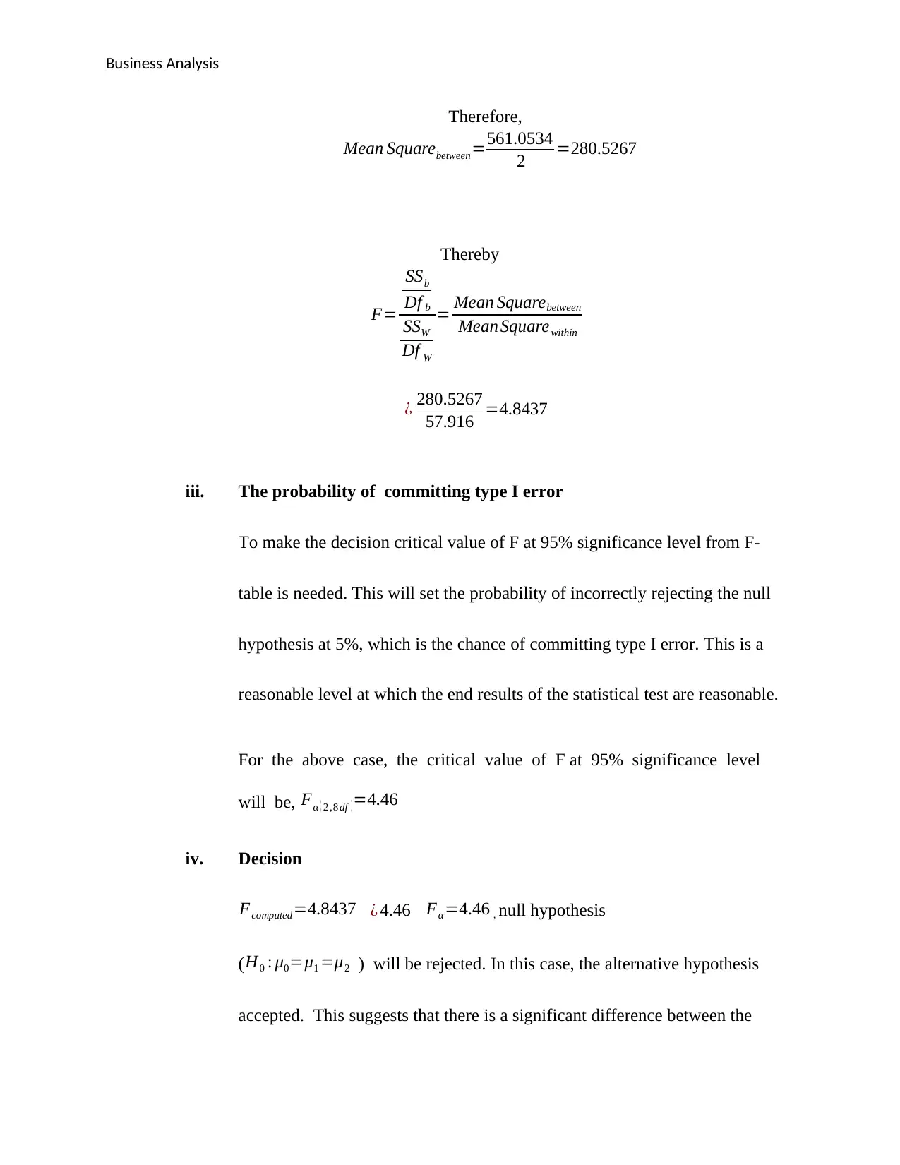
Business Analysis
Therefore,
Mean Squarebetween=561.0534
2 =280.5267
Thereby
F=
SSb
Df b
SSW
Df W
= Mean Squarebetween
Mean Squarewithin
¿ 280.5267
57.916 =4.8437
iii. The probability of committing type I error
To make the decision critical value of F at 95% significance level from F-
table is needed. This will set the probability of incorrectly rejecting the null
hypothesis at 5%, which is the chance of committing type I error. This is a
reasonable level at which the end results of the statistical test are reasonable.
For the above case, the critical value of F at 95% significance level
will be, Fα ( 2 ,8 df )=4.46
iv. Decision
Fcomputed=4.8437 ¿ 4.46 Fα =4.46 , null hypothesis
( H0 : μ0=μ1 =μ2 ) will be rejected. In this case, the alternative hypothesis
accepted. This suggests that there is a significant difference between the

Business Analysis
different Classes. This means that student’s performance is not going to be
similar, some student will do better than the other student.
In conclusion the performance of the student will be dependent on the Class
she/ he is in and the instructor of that class. This revealed by the test statistic
conducted on the data, which clearly show the existence of the difference in
the performance from different classes
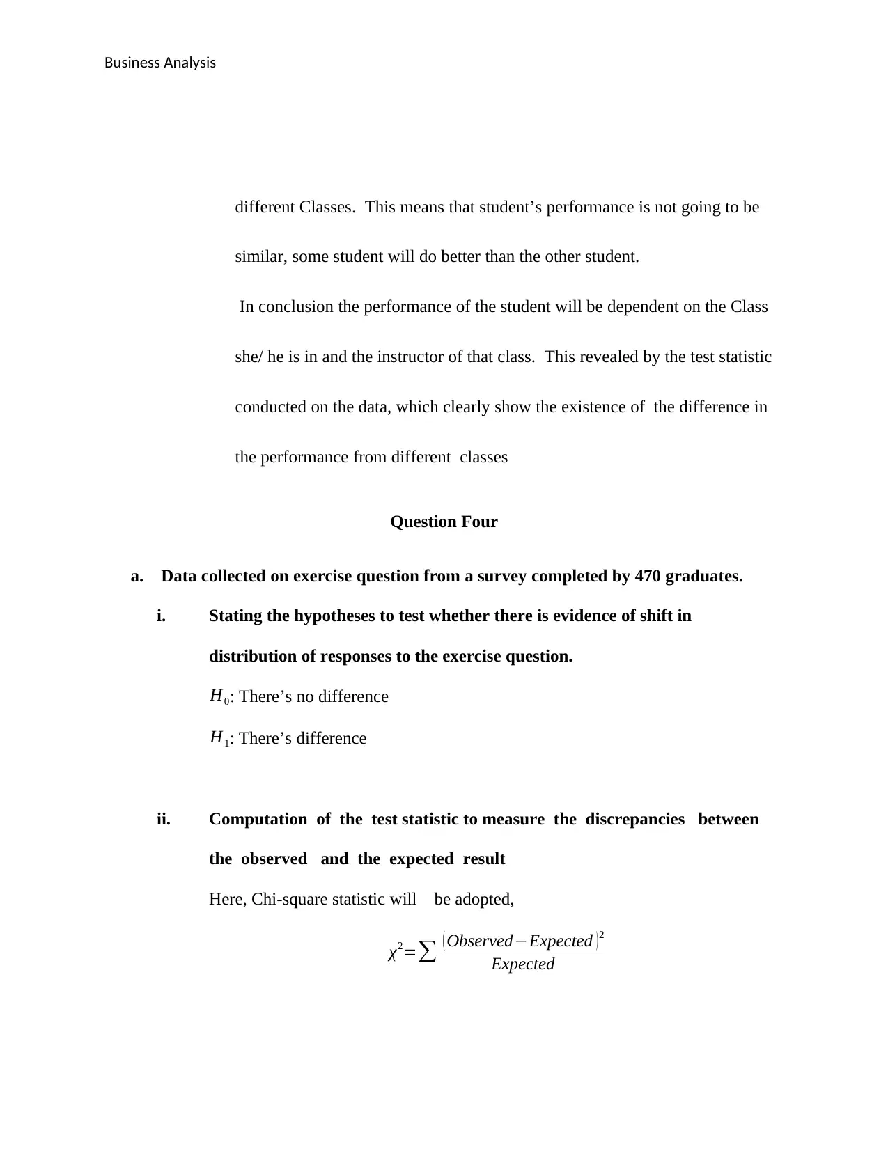
Question Four
a. Data collected on exercise question from a survey completed by 470 graduates.
i. Stating the hypotheses to test whether there is evidence of shift in
distribution of responses to the exercise question.
H0: There’s no difference
H1: There’s difference
ii. Computation of the test statistic to measure the discrepancies between
the observed and the expected result
Here, Chi-square statistic will be adopted,
χ2=∑ ( Observed−Expected )2
Expected

Business Analysis
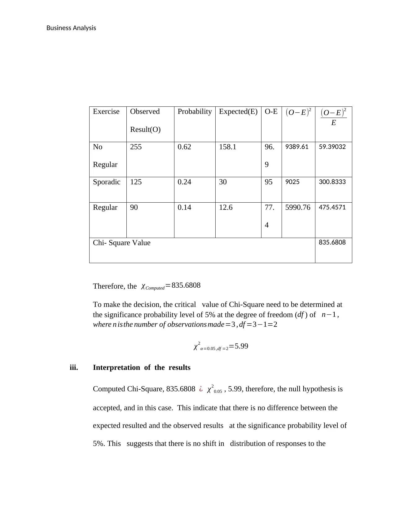
Exercise Observed
Result(O)
Probability Expected(E) O-E (O−E)2 (O−E)2
E
No
Regular
255 0.62 158.1 96.
9
9389.61 59.39032
Sporadic 125 0.24 30 95 9025 300.8333
Regular 90 0.14 12.6 77.
4
5990.76 475.4571
Chi- Square Value 835.6808
Therefore, the χComputed=835.6808
To make the decision, the critical value of Chi-Square need to be determined at
the significance probability level of 5% at the degree of freedom (df ) of n−1 ,
where n isthe number of observations made=3 , df =3−1=2
χ2
α =0.05 ,df =2=5.99
iii. Interpretation of the results
Computed Chi-Square, 835.6808 ¿ χ2
0.05 , 5.99, therefore, the null hypothesis is
accepted, and in this case. This indicate that there is no difference between the
expected resulted and the observed results at the significance probability level of
5%. This suggests that there is no shift in distribution of responses to the

Business Analysis
exercise question following the implementation of the health promotion campaign
on campus.
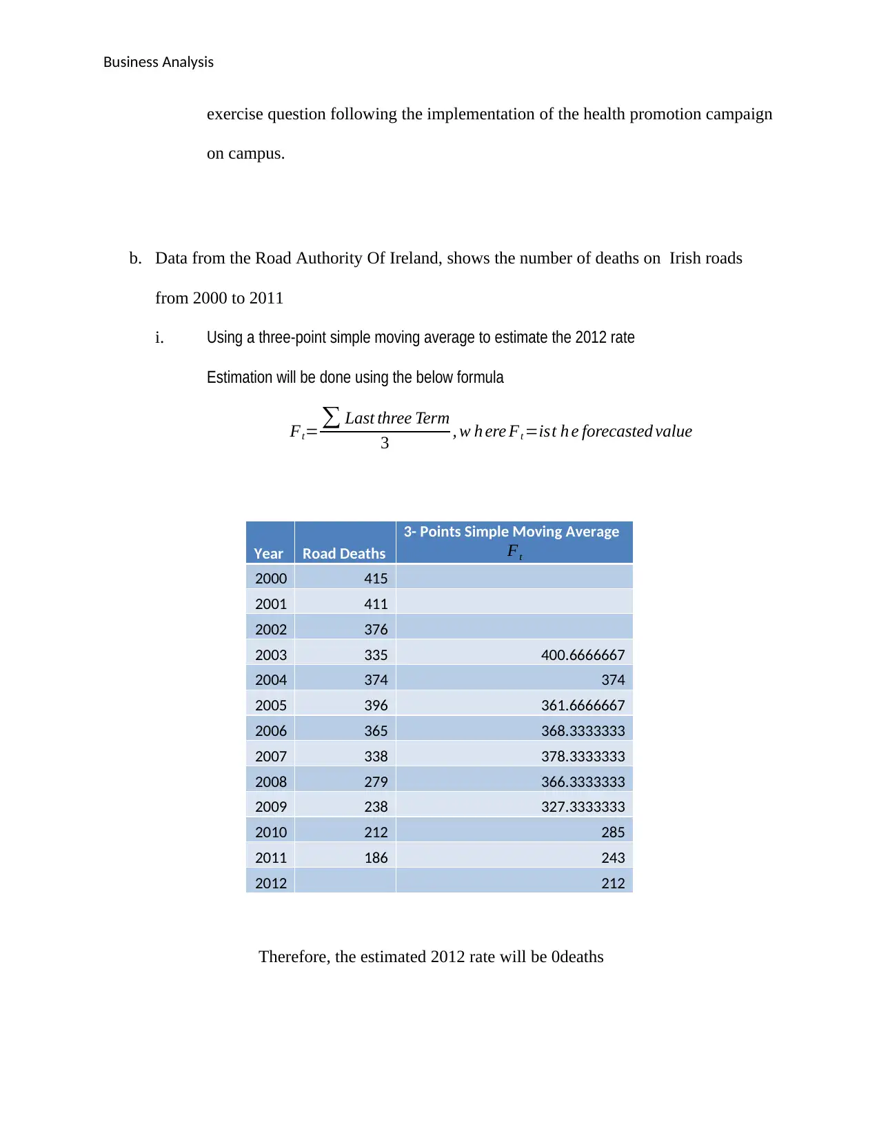
b. Data from the Road Authority Of Ireland, shows the number of deaths on Irish roads
from 2000 to 2011
i. Using a three-point simple moving average to estimate the 2012 rate
Estimation will be done using the below formula
Ft= ∑ Last three Term
3 , w h ere Ft =ist h e forecasted value
Year Road Deaths
3- Points Simple Moving Average
Ft
2000 415
2001 411
2002 376
2003 335 400.6666667
2004 374 374
2005 396 361.6666667
2006 365 368.3333333
2007 338 378.3333333
2008 279 366.3333333
2009 238 327.3333333
2010 212 285
2011 186 243
2012 212
Therefore, the estimated 2012 rate will be 0deaths