Business Data Analysis Exam: Statistical Analysis and Applications

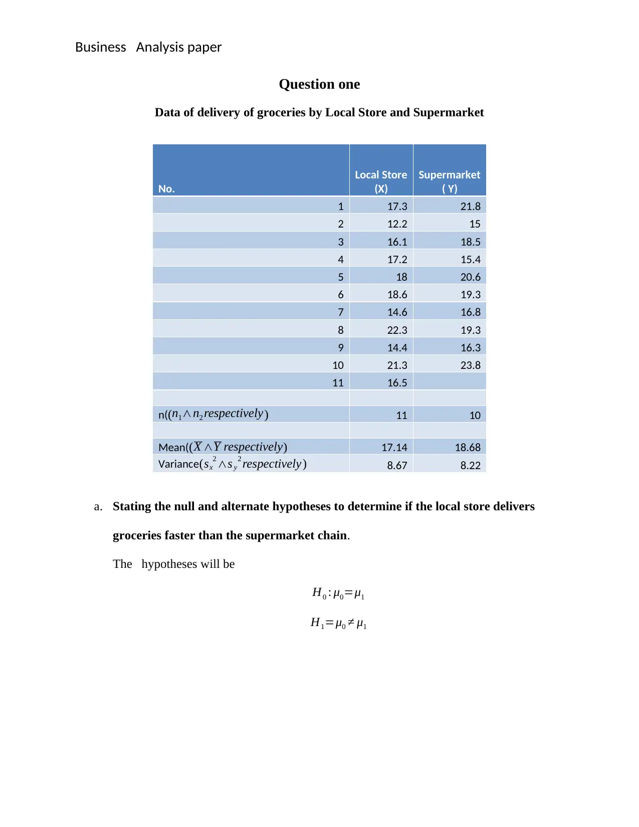
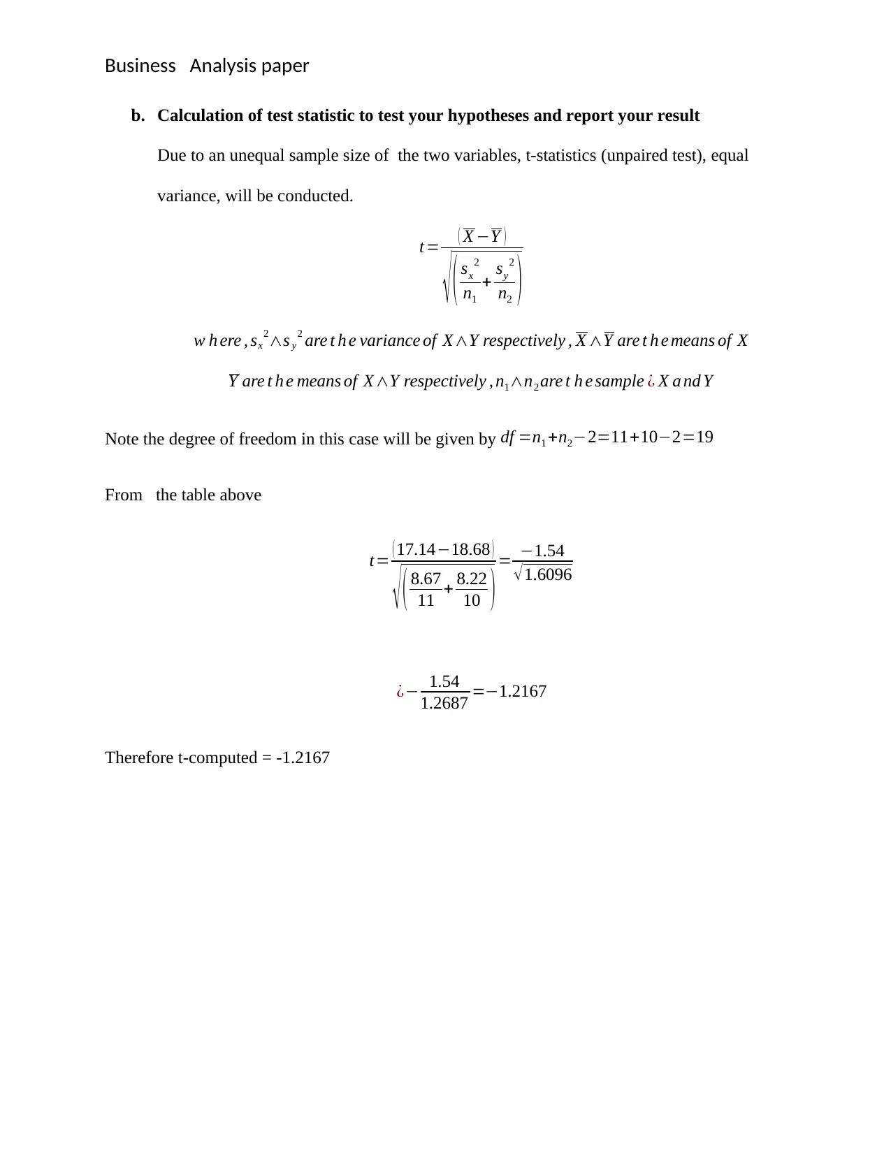
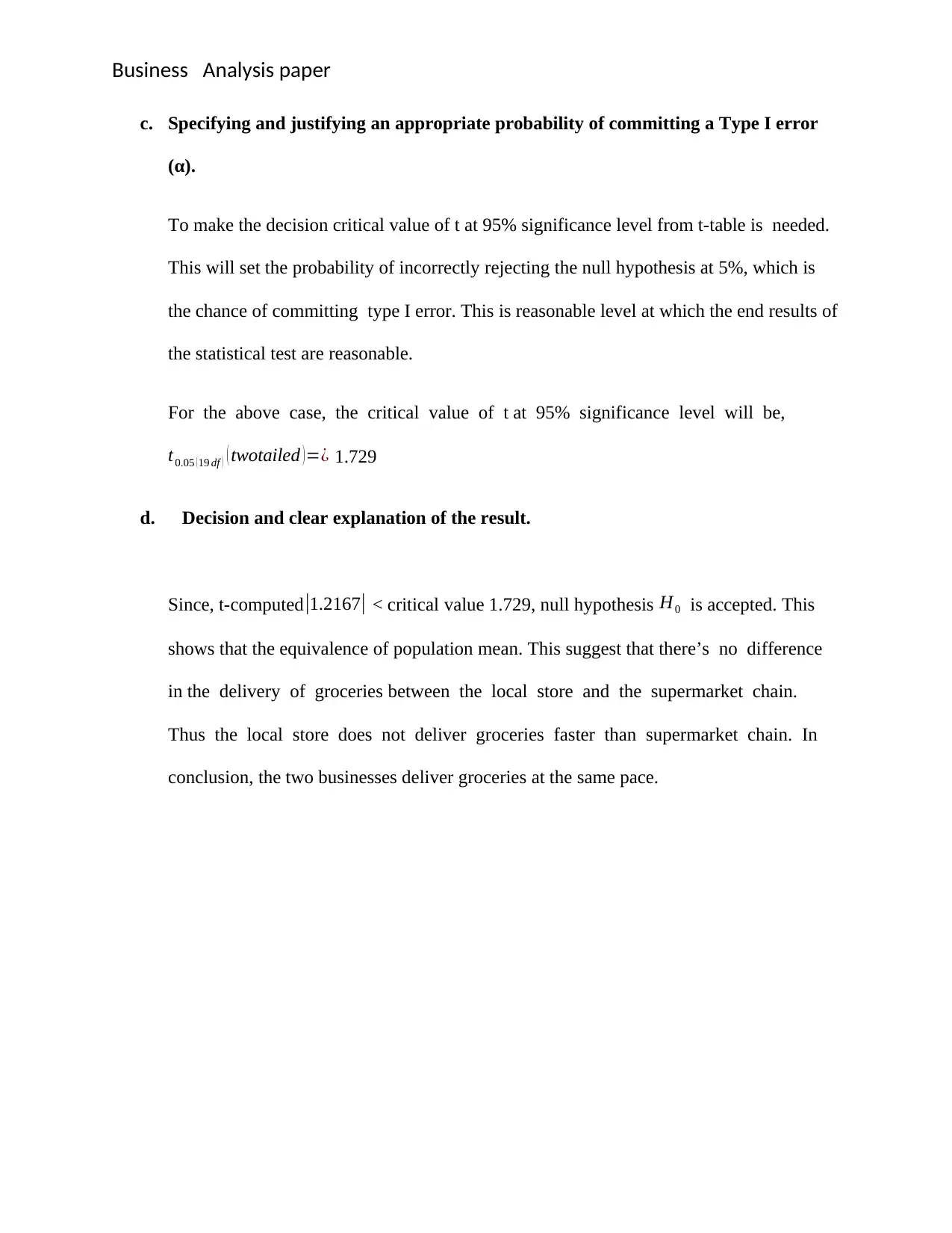
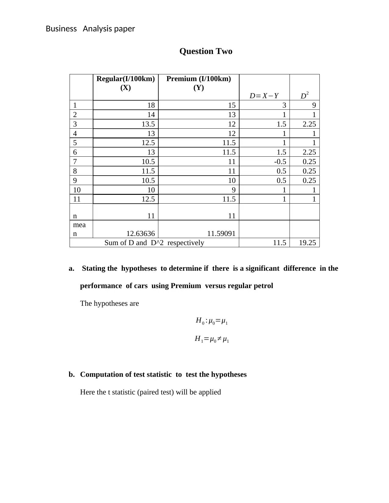
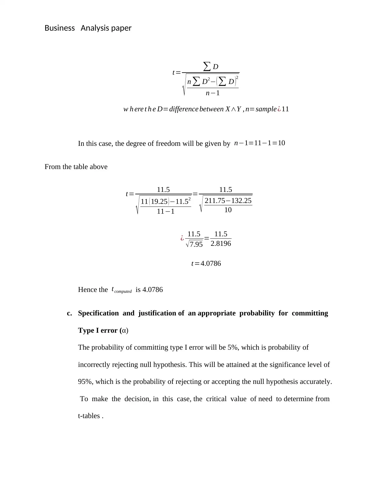
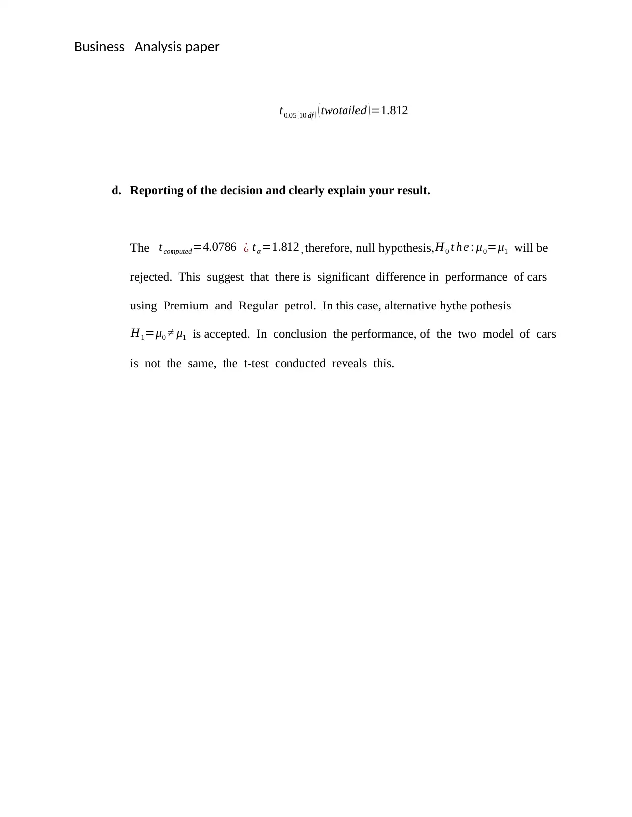
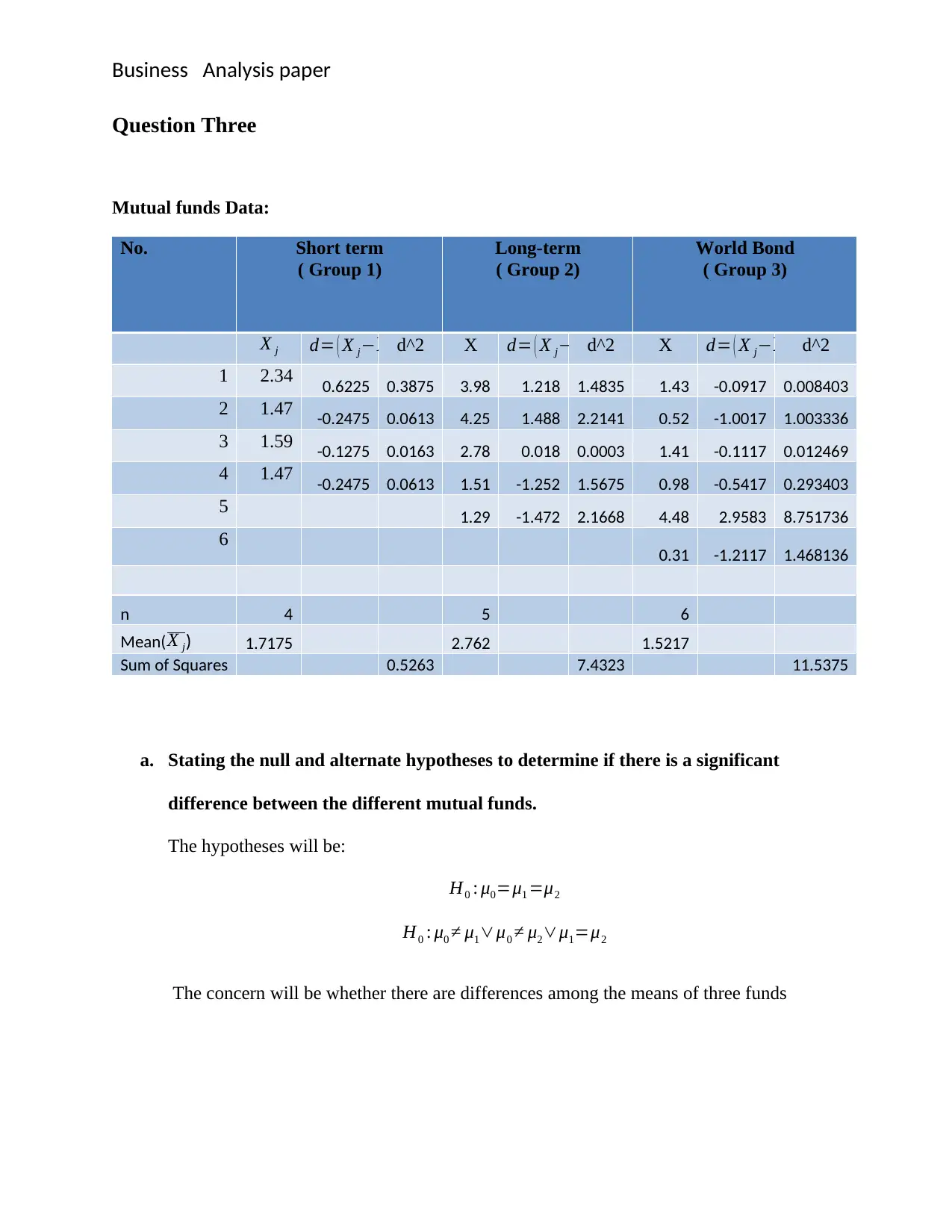
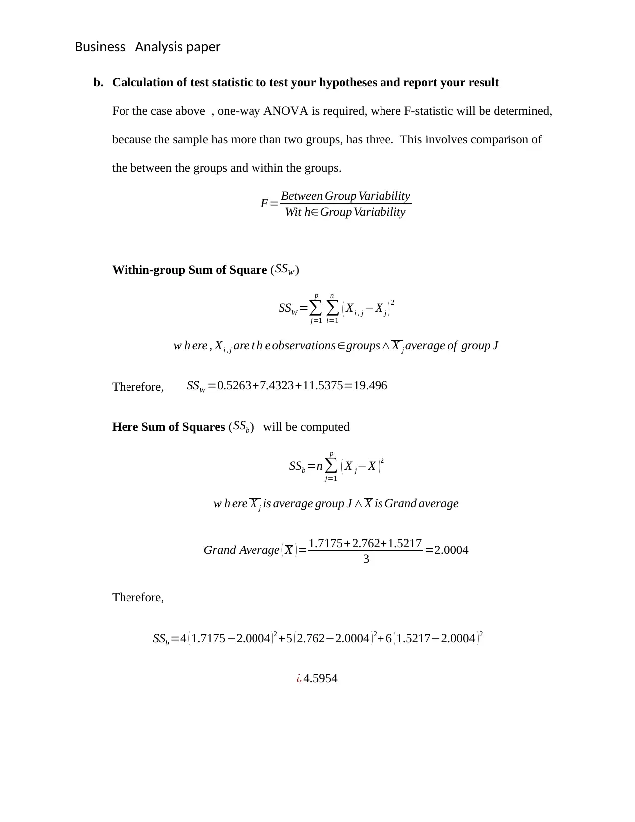
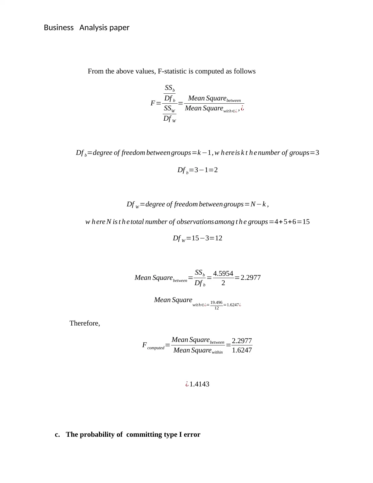
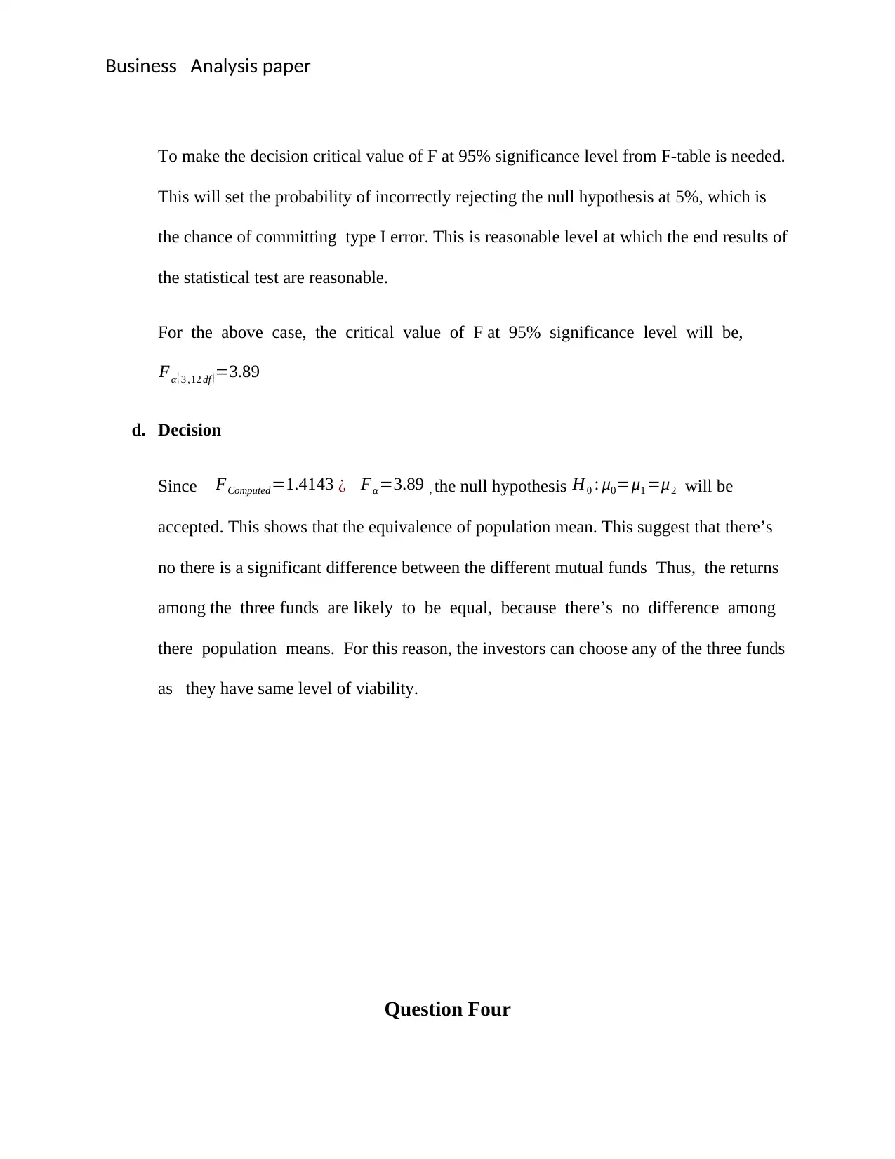
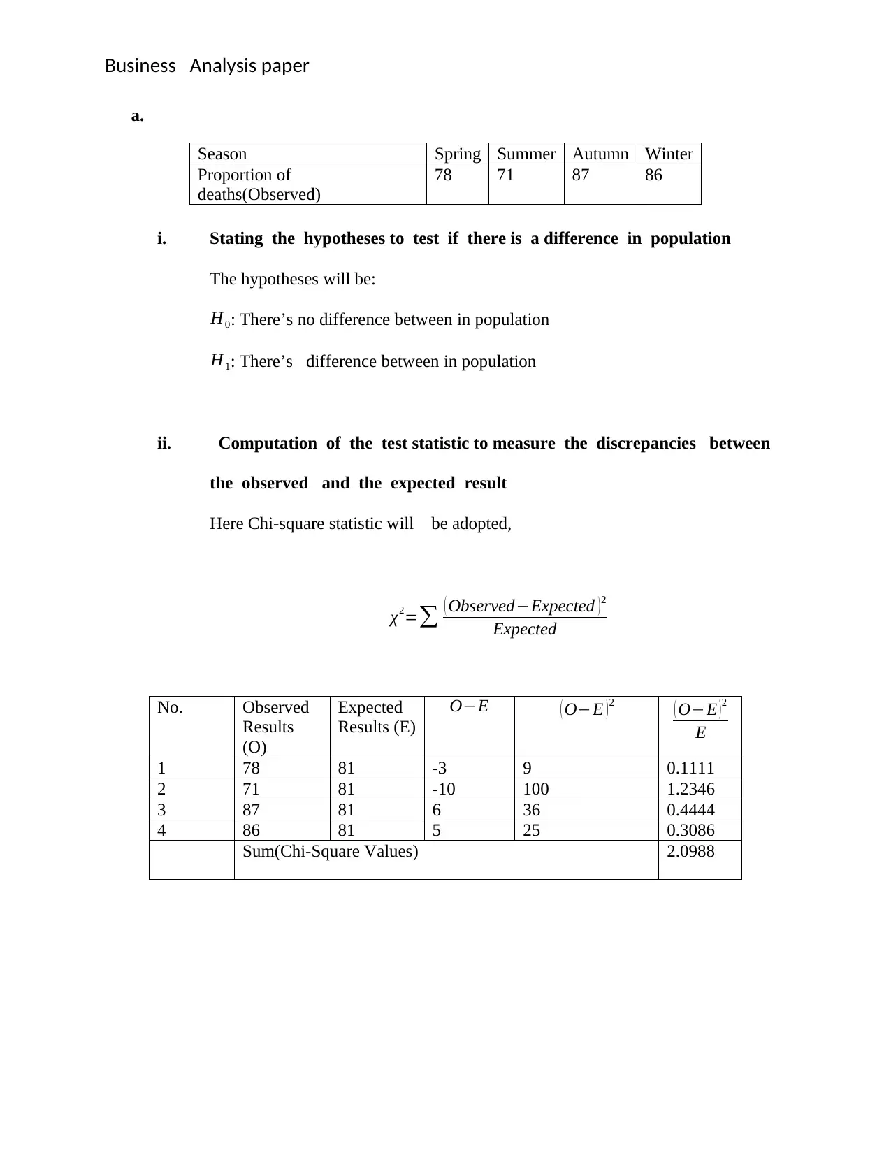
This document provides detailed solutions to a Business Data Analysis exam, covering various statistical concepts and their applications. The exam questions include hypothesis testing to compare grocery delivery times between a local store and a supermarket chain, analyzing car performance using regular versus premium petrol with paired t-tests, determining significant differences between mutual funds using one-way ANOVA, and testing population differences using the chi-square statistic. Additionally, the solutions demonstrate time series analysis techniques such as simple moving average, weighted moving average, and exponential smoothing to estimate Bitcoin closing prices. Each solution includes the null and alternative hypotheses, test statistic calculations, justification for the chosen significance level, and a clear interpretation of the results, providing a comprehensive understanding of the statistical methods applied.

Business Analysis paper
Student Name:
Course Name:
Institution Affiliation

Business Analysis paper
Question one
Data of delivery of groceries by Local Store and Supermarket
No.
Local Store
(X)
Supermarket
( Y)
1 17.3 21.8
2 12.2 15
3 16.1 18.5
4 17.2 15.4
5 18 20.6
6 18.6 19.3
7 14.6 16.8
8 22.3 19.3
9 14.4 16.3
10 21.3 23.8
11 16.5
n((n1∧n2 respectively) 11 10
Mean(( X ∧Y respectively) 17.14 18.68
Variance( sx
2 ∧s y
2 respectively) 8.67 8.22
a. Stating the null and alternate hypotheses to determine if the local store delivers
groceries faster than the supermarket chain.
The hypotheses will be
H0 : μ0=μ1
H1=μ0 ≠ μ1

Business Analysis paper
b. Calculation of test statistic to test your hypotheses and report your result
Due to an unequal sample size of the two variables, t-statistics (unpaired test), equal
variance, will be conducted.
t= ( X −Y )
√ ( sx
2
n1
+ sy
2
n2 )
w h ere , sx
2∧s y
2 are t h e variance of X∧Y respectively , X ∧Y are t h e means of X
Y are t h e means of X∧Y respectively , n1∧n2 are t h e sample ¿ X a nd Y
Note the degree of freedom in this case will be given by df =n1 +n2−2=11+10−2=19
From the table above
t= ( 17.14−18.68 )
√ ( 8.67
11 + 8.22
10 ) = −1.54
√ 1.6096
¿− 1.54
1.2687 =−1.2167
Therefore t-computed = -1.2167

Business Analysis paper
c. Specifying and justifying an appropriate probability of committing a Type I error
(α).
To make the decision critical value of t at 95% significance level from t-table is needed.
This will set the probability of incorrectly rejecting the null hypothesis at 5%, which is
the chance of committing type I error. This is reasonable level at which the end results of
the statistical test are reasonable.
For the above case, the critical value of t at 95% significance level will be,
t0.05 (19 df ) ( twotailed )=¿ 1.729
d. Decision and clear explanation of the result.
Since, t-computed |1.2167| < critical value 1.729, null hypothesis H0 is accepted. This
shows that the equivalence of population mean. This suggest that there’s no difference
in the delivery of groceries between the local store and the supermarket chain.
Thus the local store does not deliver groceries faster than supermarket chain. In
conclusion, the two businesses deliver groceries at the same pace.

Business Analysis paper
Question Two
Regular(I/100km)
(X)
Premium (I/100km)
(Y)
D= X−Y D2
1 18 15 3 9
2 14 13 1 1
3 13.5 12 1.5 2.25
4 13 12 1 1
5 12.5 11.5 1 1
6 13 11.5 1.5 2.25
7 10.5 11 -0.5 0.25
8 11.5 11 0.5 0.25
9 10.5 10 0.5 0.25
10 10 9 1 1
11 12.5 11.5 1 1
n 11 11
mea
n 12.63636 11.59091
Sum of D and D^2 respectively 11.5 19.25
a. Stating the hypotheses to determine if there is a significant difference in the
performance of cars using Premium versus regular petrol
The hypotheses are
H0 : μ0=μ1
H1=μ0 ≠ μ1
b. Computation of test statistic to test the hypotheses
Here the t statistic (paired test) will be applied

Business Analysis paper
t= ∑ D
√ n ∑ D2− ( ∑ D )
2
n−1
w h ere t h e D=difference between X∧Y , n=sample ¿ 11
In this case, the degree of freedom will be given by n−1=11−1=10
From the table above
t= 11.5
√ 11 ( 19.25 )−11.52
11−1
= 11.5
√ 211.75−132.25
10
¿ 11.5
√7.95 = 11.5
2.8196
t=4.0786
Hence the tcomputed is 4.0786
c. Specification and justification of an appropriate probability for committing
Type I error (α)
The probability of committing type I error will be 5%, which is probability of
incorrectly rejecting null hypothesis. This will be attained at the significance level of
95%, which is the probability of rejecting or accepting the null hypothesis accurately.
To make the decision, in this case, the critical value of need to determine from
t-tables .

Business Analysis paper
t0.05 ( 10 df ) ( twotailed ) =1.812
d. Reporting of the decision and clearly explain your result.
The tcomputed=4.0786 ¿ tα=1.812 , therefore, null hypothesis,H0 t h e : μ0=μ1 will be
rejected. This suggest that there is significant difference in performance of cars
using Premium and Regular petrol. In this case, alternative hythe pothesis
H1=μ0 ≠ μ1 is accepted. In conclusion the performance, of the two model of cars
is not the same, the t-test conducted reveals this.

Business Analysis paper
Question Three
Mutual funds Data:
No. Short term
( Group 1)
Long-term
( Group 2)
World Bond
( Group 3)
X j d= ( X j−X j )d^2 X d= ( X j−X j )d^2 X d= ( X j−X j ) d^2
1 2.34 0.6225 0.3875 3.98 1.218 1.4835 1.43 -0.0917 0.008403
2 1.47 -0.2475 0.0613 4.25 1.488 2.2141 0.52 -1.0017 1.003336
3 1.59 -0.1275 0.0163 2.78 0.018 0.0003 1.41 -0.1117 0.012469
4 1.47 -0.2475 0.0613 1.51 -1.252 1.5675 0.98 -0.5417 0.293403
5 1.29 -1.472 2.1668 4.48 2.9583 8.751736
6 0.31 -1.2117 1.468136
n 4 5 6
Mean( X j) 1.7175 2.762 1.5217
Sum of Squares 0.5263 7.4323 11.5375
a. Stating the null and alternate hypotheses to determine if there is a significant
difference between the different mutual funds.
The hypotheses will be:
H0 : μ0=μ1 =μ2
H0 : μ0 ≠ μ1∨μ0 ≠ μ2∨μ1=μ2
The concern will be whether there are differences among the means of three funds

Business Analysis paper
b. Calculation of test statistic to test your hypotheses and report your result
For the case above , one-way ANOVA is required, where F-statistic will be determined,
because the sample has more than two groups, has three. This involves comparison of
the between the groups and within the groups.
F= Between Group Variability
Wit h∈Group Variability
Within-group Sum of Square ( SSW )
SSW =∑
j=1
p
∑
i=1
n
( Xi , j −X j ) 2
w h ere , Xi , j are t h e observations∈groups∧X j average of group J
Therefore, SSW =0.5263+7.4323+11.5375=19.496
Here Sum of Squares (SSb) will be computed
SSb =n∑
j=1
p
( X j−X )2
w h ere X j is average group J ∧X is Grand average
Grand Average ( X )=1.7175+ 2.762+1.5217
3 =2.0004
Therefore,
SSb =4 ( 1.7175−2.0004 )2 +5 ( 2.762−2.0004 )2+ 6 ( 1.5217−2.0004 )2
¿ 4.5954

Business Analysis paper
From the above values, F-statistic is computed as follows
F=
SSb
Df b
SSW
Df W
= Mean Squarebetween
Mean Squarewit h ∈¿ , ¿
Df b=degree of freedom between groups=k −1, w h ereis k t h e number of groups=3
Df b=3−1=2
Df W =degree of freedom between groups=N−k ,
w h ere N is t h e total number of observations among t h e groups=4+5+6=15
Df W =15−3=12
Mean Squarebetween = SSb
Df b
= 4.5954
2 =2.2977
Mean Squarewit h ∈¿= 19.496
12 =1.6247¿
Therefore,
Fcomputed= Mean Squarebetween
Mean Squarewithin
=2.2977
1.6247
¿ 1.4143
c. The probability of committing type I error

Business Analysis paper
To make the decision critical value of F at 95% significance level from F-table is needed.
This will set the probability of incorrectly rejecting the null hypothesis at 5%, which is
the chance of committing type I error. This is reasonable level at which the end results of
the statistical test are reasonable.
For the above case, the critical value of F at 95% significance level will be,
Fα ( 3 ,12 df )=3.89
d. Decision
Since FComputed=1.4143 ¿ Fα =3.89 , the null hypothesis H0 : μ0=μ1 =μ2 will be
accepted. This shows that the equivalence of population mean. This suggest that there’s
no there is a significant difference between the different mutual funds Thus, the returns
among the three funds are likely to be equal, because there’s no difference among
there population means. For this reason, the investors can choose any of the three funds
as they have same level of viability.
Question Four

Business Analysis paper
a.
Season Spring Summer Autumn Winter
Proportion of
deaths(Observed)
78 71 87 86
i. Stating the hypotheses to test if there is a difference in population
The hypotheses will be:
H0: There’s no difference between in population
H1: There’s difference between in population
ii. Computation of the test statistic to measure the discrepancies between
the observed and the expected result
Here Chi-square statistic will be adopted,
χ2=∑ ( Observed−Expected )2
Expected
No. Observed
Results
(O)
Expected
Results (E)
O−E ( O−E )2 ( O−E ) 2
E
1 78 81 -3 9 0.1111
2 71 81 -10 100 1.2346
3 87 81 6 36 0.4444
4 86 81 5 25 0.3086
Sum(Chi-Square Values) 2.0988