Decision Analysis and Support Tools for Business Development

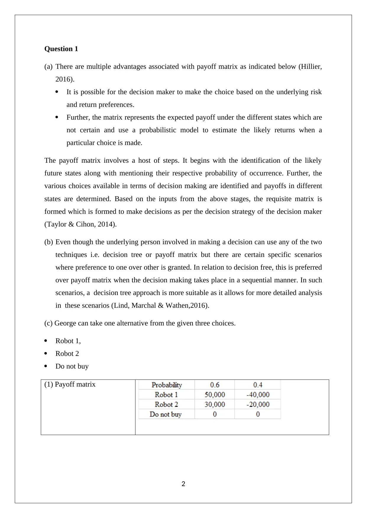
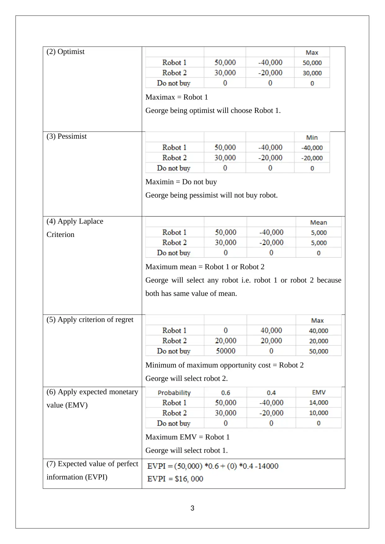
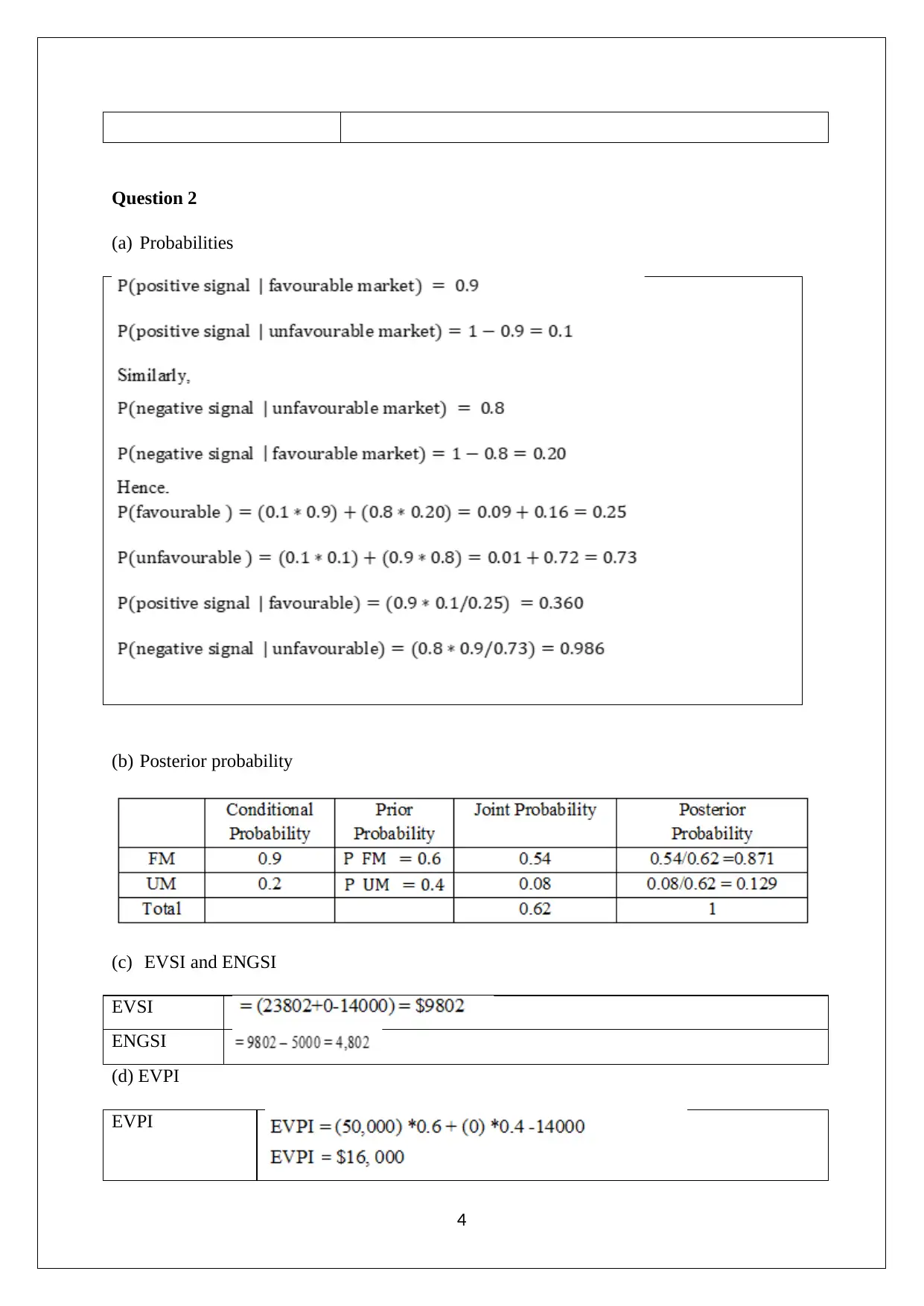
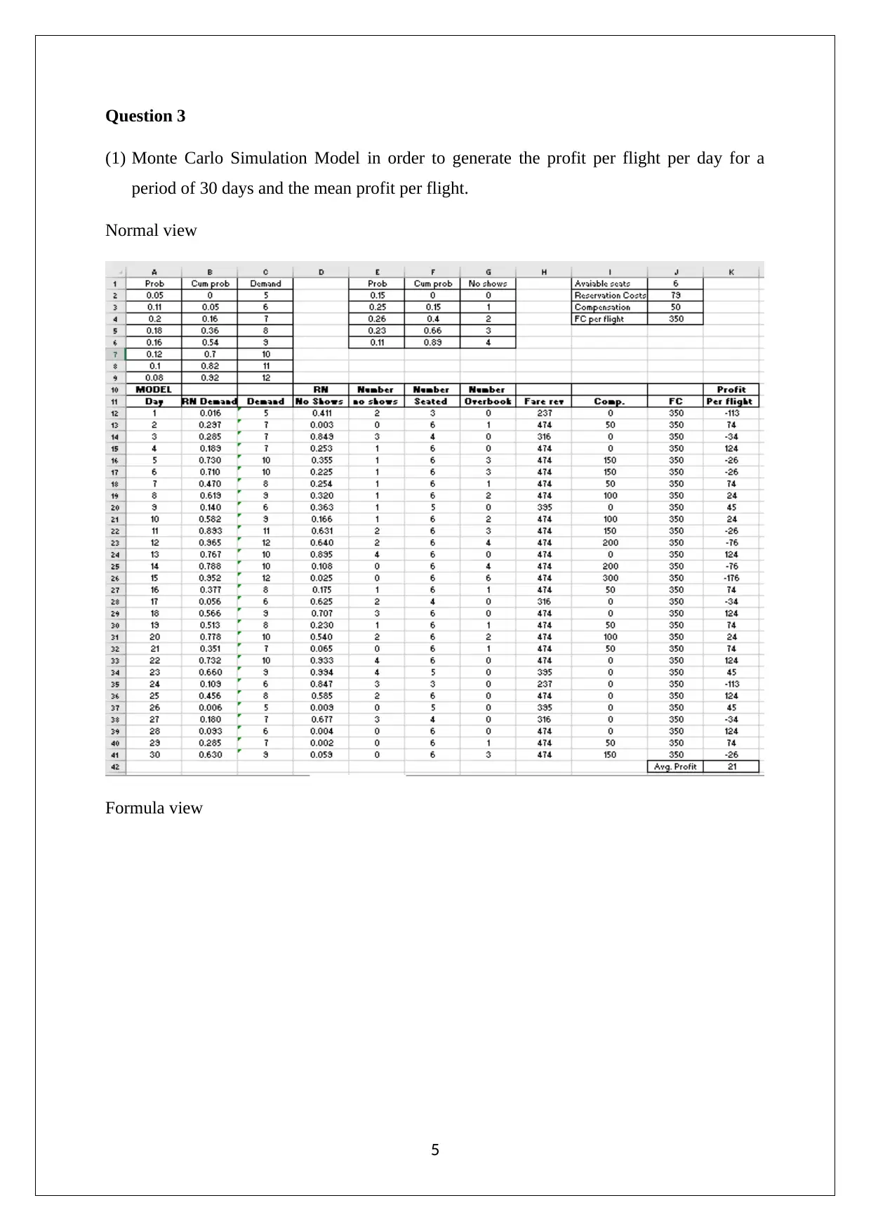
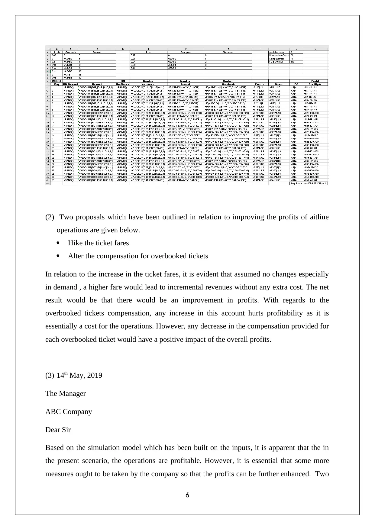
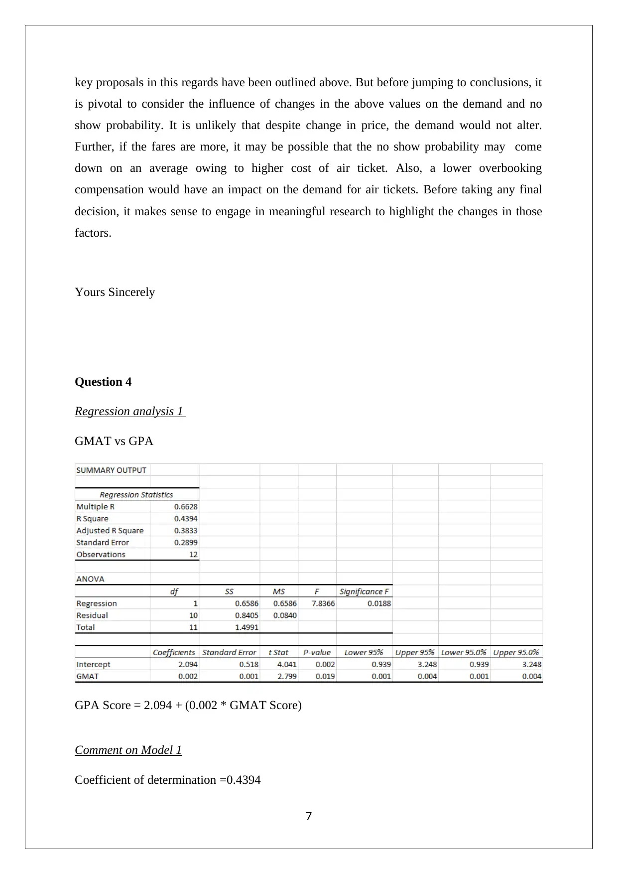
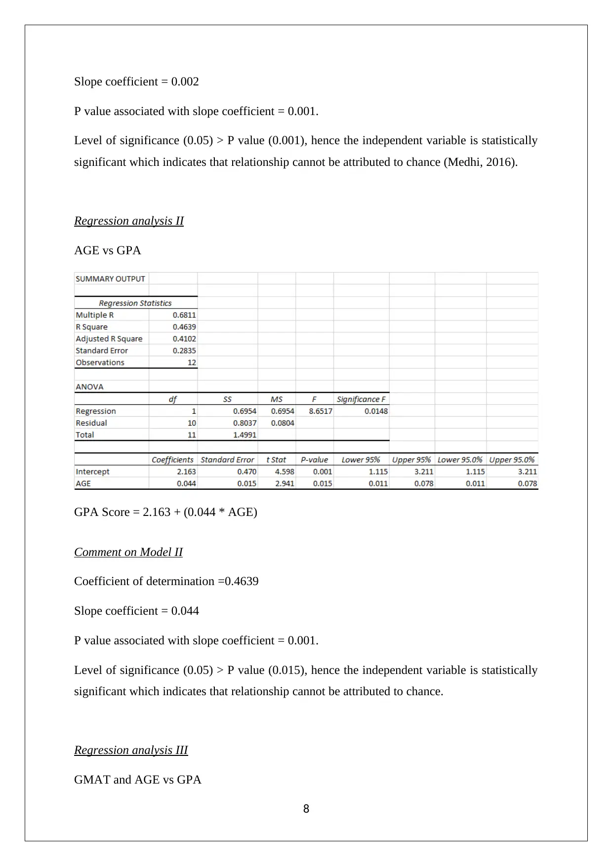
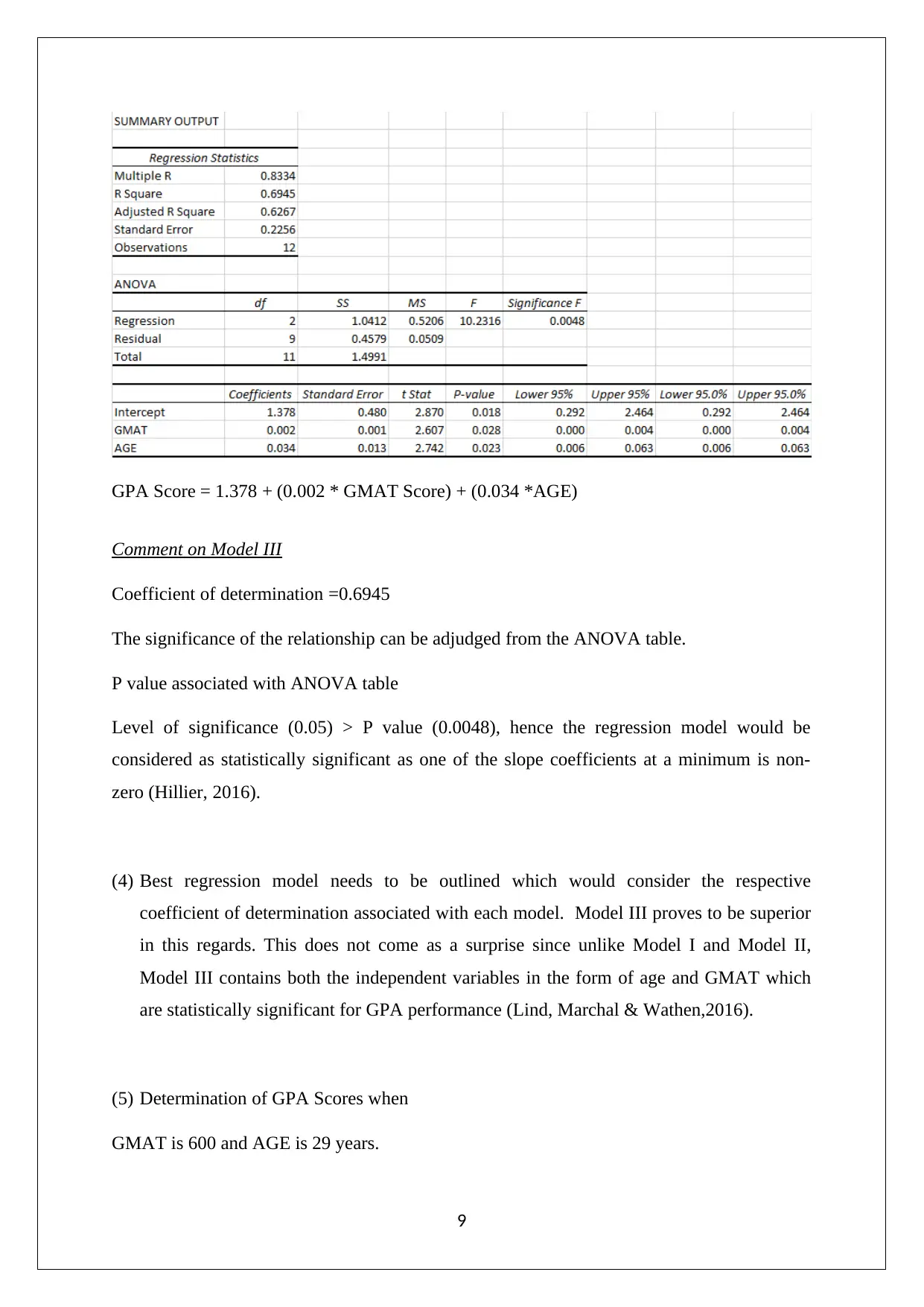
This assignment provides a comprehensive analysis of decision support tools. It begins by discussing the advantages and steps involved in using a payoff matrix, followed by a comparison with decision trees, highlighting scenarios where each is preferred. The assignment then applies various decision-making criteria, such as optimist, pessimist, Laplace criterion, regret criterion, and expected monetary value, to a practical problem involving robot purchases. Further, it delves into probability analysis, including posterior probabilities, EVSI, ENGSI, and EVPI. The assignment also utilizes Monte Carlo simulation to model profit per flight and proposes strategies to improve airline profitability, such as adjusting ticket fares and overbooking compensation. Finally, it conducts regression analysis to assess the relationship between GMAT scores, age, and GPA, identifying the best-fit model and predicting GPA scores based on given parameters, and break even analysis. The document is available on Desklib, a platform offering a wide range of study resources for students.

DECISION SUPPORT TOOLS
STUDENT ID:
[Pick the date]

Question 1
(a) There are multiple advantages associated with payoff matrix as indicated below (Hillier,
2016).
 It is possible for the decision maker to make the choice based on the underlying risk
and return preferences.
 Further, the matrix represents the expected payoff under the different states which are
not certain and use a probabilistic model to estimate the likely returns when a
particular choice is made.
The payoff matrix involves a host of steps. It begins with the identification of the likely
future states along with mentioning their respective probability of occurrence. Further, the
various choices available in terms of decision making are identified and payoffs in different
states are determined. Based on the inputs from the above stages, the requisite matrix is
formed which is formed to make decisions as per the decision strategy of the decision maker
(Taylor & Cihon, 2014).
(b) Even though the underlying person involved in making a decision can use any of the two
techniques i.e. decision tree or payoff matrix but there are certain specific scenarios
where preference to one over other is granted. In relation to decision free, this is preferred
over payoff matrix when the decision making takes place in a sequential manner. In such
scenarios, a decision tree approach is more suitable as it allows for more detailed analysis
in these scenarios (Lind, Marchal & Wathen,2016).
(c) George can take one alternative from the given three choices.
 Robot 1,
 Robot 2
 Do not buy
(1) Payoff matrix
2

(2) Optimist
Maximax = Robot 1
George being optimist will choose Robot 1.
(3) Pessimist
Maximin = Do not buy
George being pessimist will not buy robot.
(4) Apply Laplace
Criterion
Maximum mean = Robot 1 or Robot 2
George will select any robot i.e. robot 1 or robot 2 because
both has same value of mean.
(5) Apply criterion of regret
Minimum of maximum opportunity cost = Robot 2
George will select robot 2.
(6) Apply expected monetary
value (EMV)
Maximum EMV = Robot 1
George will select robot 1.
(7) Expected value of perfect
information (EVPI)
3

Question 2
(a) Probabilities
(b) Posterior probability
(c) EVSI and ENGSI
EVSI
ENGSI
(d) EVPI
EVPI
4

Question 3
(1) Monte Carlo Simulation Model in order to generate the profit per flight per day for a
period of 30 days and the mean profit per flight.
Normal view
Formula view
5

(2) Two proposals which have been outlined in relation to improving the profits of aitline
operations are given below.
 Hike the ticket fares
 Alter the compensation for overbooked tickets
In relation to the increase in the ticket fares, it is evident that assumed no changes especially
in demand , a higher fare would lead to incremental revenues without any extra cost. The net
result would be that there would be an improvement in profits. With regards to the
overbooked tickets compensation, any increase in this account hurts profitability as it is
essentially a cost for the operations. However, any decrease in the compensation provided for
each overbooked ticket would have a positive impact of the overall profits.
(3) 14th May, 2019
The Manager
ABC Company
Dear Sir
Based on the simulation model which has been built on the inputs, it is apparent that the in
the present scenario, the operations are profitable. However, it is essential that some more
measures ought to be taken by the company so that the profits can be further enhanced. Two
6

key proposals in this regards have been outlined above. But before jumping to conclusions, it
is pivotal to consider the influence of changes in the above values on the demand and no
show probability. It is unlikely that despite change in price, the demand would not alter.
Further, if the fares are more, it may be possible that the no show probability may come
down on an average owing to higher cost of air ticket. Also, a lower overbooking
compensation would have an impact on the demand for air tickets. Before taking any final
decision, it makes sense to engage in meaningful research to highlight the changes in those
factors.
Yours Sincerely
Question 4
Regression analysis 1
GMAT vs GPA
GPA Score = 2.094 + (0.002 * GMAT Score)
Comment on Model 1
Coefficient of determination =0.4394
7

Slope coefficient = 0.002
P value associated with slope coefficient = 0.001.
Level of significance (0.05) > P value (0.001), hence the independent variable is statistically
significant which indicates that relationship cannot be attributed to chance (Medhi, 2016).
Regression analysis II
AGE vs GPA
GPA Score = 2.163 + (0.044 * AGE)
Comment on Model II
Coefficient of determination =0.4639
Slope coefficient = 0.044
P value associated with slope coefficient = 0.001.
Level of significance (0.05) > P value (0.015), hence the independent variable is statistically
significant which indicates that relationship cannot be attributed to chance.
Regression analysis III
GMAT and AGE vs GPA
8

GPA Score = 1.378 + (0.002 * GMAT Score) + (0.034 *AGE)
Comment on Model III
Coefficient of determination =0.6945
The significance of the relationship can be adjudged from the ANOVA table.
P value associated with ANOVA table
Level of significance (0.05) > P value (0.0048), hence the regression model would be
considered as statistically significant as one of the slope coefficients at a minimum is non-
zero (Hillier, 2016).
(4) Best regression model needs to be outlined which would consider the respective
coefficient of determination associated with each model. Model III proves to be superior
in this regards. This does not come as a surprise since unlike Model I and Model II,
Model III contains both the independent variables in the form of age and GMAT which
are statistically significant for GPA performance (Lind, Marchal & Wathen,2016).
(5) Determination of GPA Scores when
GMAT is 600 and AGE is 29 years.
9

Applicable regression equation
Hence,
Question 5
(1) Break-even units and the corresponding dollars
(2) Units to derive a targeted profit before tax as $600
(3) Computation of profit when there is 250 units are available for sale
(4) Product A and product B units and dollars
Assuming that the product A’s unit is 2X and product B’s unit is X.
Now, Contribution margin for product B
10

Further, Profit before tax
Gross profit (As a whole for both products) = 24 X
Product A units and dollars =2*x = 2*300 =600 units
= (600*12) = $7200
Product B units and dollars =x = 300 =300 units
= (300*20) = $6000
11

References
Hillier, F. (2016).Introduction to Operations Research.(6thed.). New York: McGraw Hill
Publications.
Lind, A.D., Marchal, G.W. &Wathen, A.S. (2016).Statistical Techniques in Business and
Economics (15thed.). New York : McGraw-Hill/Irwin.
Medhi, J. (2016). Statistical Methods: An Introductory Text (4thed.). Sydney: New Age
International.
Taylor, K. J. & Cihon, C. (2014).Statistical Techniques for Data Analysis (2nded.).
Melbourne: CRC Press.
12