Business Analytics and Decision Modelling Report: Predicting Profits

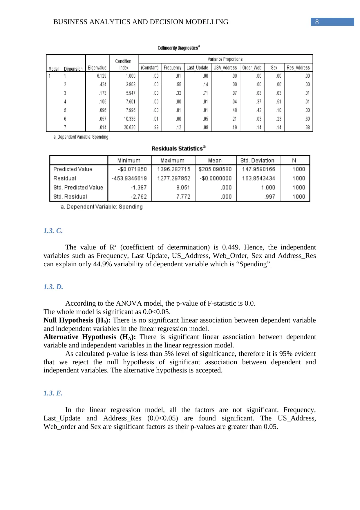
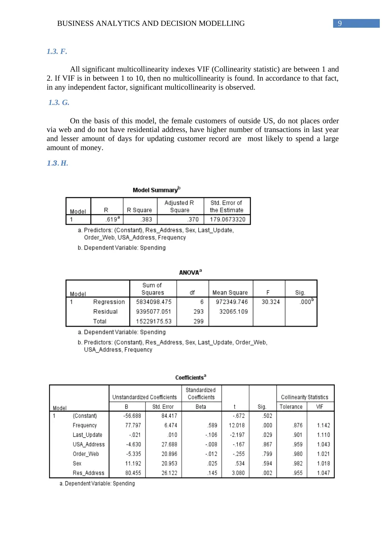
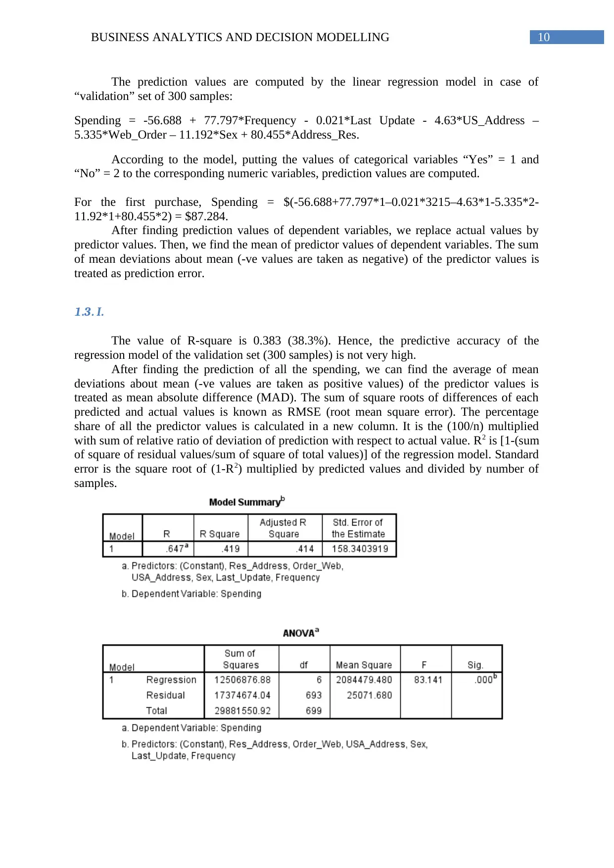
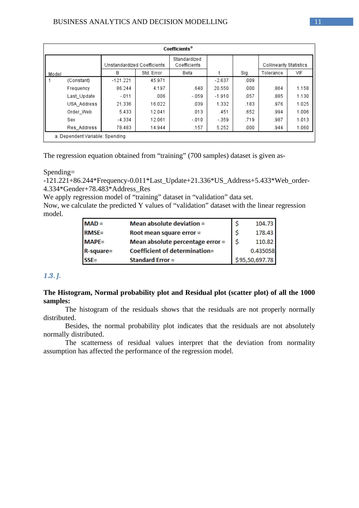
This report, focusing on Business Analytics and Decision Modeling, presents an analysis of two key areas: predicting software reselling profits and examining housing price structures. The profit prediction section employs exploratory statistics, scatter plots, and linear regression models to determine factors influencing customer spending. The analysis includes randomization, preprocessing of categorical variables, and evaluation of model significance, multicollinearity, and predictive accuracy. The second part investigates housing price structures in a specific township using one-sample and two-sample t-tests to assess premium prices for brick houses and different neighborhoods. The report explores hypotheses, test results, and interpretations, including the transformation of neighborhood levels for estimation purposes. The analysis uses statistical tools to evaluate the relationship between different variables and their impact on business decisions.

Running head: BUSINESS ANALYTICS AND DECISION MODELLING
Business Analytics and Decision Modelling
Name of the Student:
Name of the University:
Author’s Note:

1BUSINESS ANALYTICS AND DECISION MODELLING
Table of Contents
1. Predicting Software Reselling Profits....................................................................................2
1.1. Exploratory Statistics:.....................................................................................................2
1.2. Scatter plot:.....................................................................................................................4
1.2.1. Freq vs. Spending scatter plot:.................................................................................4
1.2.2. Last Update vs. Spending scatter plot:.....................................................................5
1.3. Prediction of Spending:...................................................................................................5
1.3. A. Randomization of the samples and Preprocessing of categorical variables:..........5
1.3. B. Linear Regression Model:......................................................................................6
1.3. C..................................................................................................................................7
1.3. D..................................................................................................................................7
1.3. E..................................................................................................................................7
1.3. F...................................................................................................................................8
1.3. G..................................................................................................................................8
1.3. H..................................................................................................................................8
1.3. I...................................................................................................................................8
1.3. J...................................................................................................................................8
2. Housing Price Structure in “NOTAREAL” Township:.......................................................11
2.1. One sample t-test:..........................................................................................................11
2.2. One sample t-test:..........................................................................................................12

2BUSINESS ANALYTICS AND DECISION MODELLING
2.3. Two Sample and Independent Sample t-test:................................................................12
2.4. Transformation of level of Neighbourhood:.................................................................15
Annotated Bibliography:..........................................................................................................16

3BUSINESS ANALYTICS AND DECISION MODELLING
1. Predicting Software Reselling Profits
1.1. Exploratory Statistics:
US address vs. Spending
Out of 1000 samples, 167 customers dwell in US whose average spending is $213 with
standard deviation $201. Rest 833 customers who do not have US address have average
spending $204 with standard deviation $225.
Web Order vs. Spending:
Out of 1000 samples, 456 customers who did not place at least one order via web have
average spending $208 with standard deviation $223. Rest 544 customers who placed at least
one order via web have average spending $202 with standard deviation $219.
Gender vs. Spending:

4BUSINESS ANALYTICS AND DECISION MODELLING
Among 1000 customers, 486 female customers spend an average amount of $210 with
standard deviation $223. 514 male customers spend an average amount of $201 with standard
deviation $219.
Addrress_res vs. Spending:
Among 1000 customers, 777 customers whose address is a not residence spend an average
amount of $211 with standard deviation $240. 223 customers whose address is a residence
spend an average amount of $185 with standard deviation $133.

5BUSINESS ANALYTICS AND DECISION MODELLING
1.2. Scatter plot:
1.2.1. Freq vs. Spending scatter plot:
The scatter plot takes into account “Number of transactions in last year at source catalogue”
as independent and “Spending” as dependent variable. The fitted trend line indicates that the
fitting of linear regression is moderately good. A moderately strong linear association is
present.

6BUSINESS ANALYTICS AND DECISION MODELLING
1.2.2. Last Update vs. Spending scatter plot:
The scatter plot takes into account “How many days ago was last update to customer record”
as independent and “Spending” as dependent variable. The fitted trend line indicates that the
fitting of linear regression is not good at all. Hence, no linear relationship exists.
1.3. Prediction of Spending:
1.3. A. Randomization of the samples and Preprocessing of categorical variables:

7BUSINESS ANALYTICS AND DECISION MODELLING
The number of “Training” samples is 700 whereas the number of “validation” sample is 300.
1.3. B. Linear Regression Model:

8BUSINESS ANALYTICS AND DECISION MODELLING
1.3. C.
The value of R2 (coefficient of determination) is 0.449. Hence, the independent
variables such as Frequency, Last Update, US_Address, Web_Order, Sex and Address_Res
can explain only 44.9% variability of dependent variable which is “Spending”.
1.3. D.
According to the ANOVA model, the p-value of F-statistic is 0.0.
The whole model is significant as 0.0<0.05.
Null Hypothesis (H0): There is no significant linear association between dependent variable
and independent variables in the linear regression model.
Alternative Hypothesis (HA): There is significant linear association between dependent
variable and independent variables in the linear regression model.
As calculated p-value is less than 5% level of significance, therefore it is 95% evident
that we reject the null hypothesis of significant association between dependent and
independent variables. The alternative hypothesis is accepted.
1.3. E.
In the linear regression model, all the factors are not significant. Frequency,
Last_Update and Address_Res (0.0<0.05) are found significant. The US_Address,
Web_order and Sex are significant factors as their p-values are greater than 0.05.

9BUSINESS ANALYTICS AND DECISION MODELLING
1.3. F.
All significant multicollinearity indexes VIF (Collinearity statistic) are between 1 and
2. If VIF is in between 1 to 10, then no multicollinearity is found. In accordance to that fact,
in any independent factor, significant multicollinearity is observed.
1.3. G.
On the basis of this model, the female customers of outside US, do not places order
via web and do not have residential address, have higher number of transactions in last year
and lesser amount of days for updating customer record are most likely to spend a large
amount of money.
1.3. H.

10BUSINESS ANALYTICS AND DECISION MODELLING
The prediction values are computed by the linear regression model in case of
“validation” set of 300 samples:
Spending = -56.688 + 77.797*Frequency - 0.021*Last Update - 4.63*US_Address –
5.335*Web_Order – 11.192*Sex + 80.455*Address_Res.
According to the model, putting the values of categorical variables “Yes” = 1 and
“No” = 2 to the corresponding numeric variables, prediction values are computed.
For the first purchase, Spending = $(-56.688+77.797*1–0.021*3215–4.63*1-5.335*2-
11.92*1+80.455*2) = $87.284.
After finding prediction values of dependent variables, we replace actual values by
predictor values. Then, we find the mean of predictor values of dependent variables. The sum
of mean deviations about mean (-ve values are taken as negative) of the predictor values is
treated as prediction error.
1.3. I.
The value of R-square is 0.383 (38.3%). Hence, the predictive accuracy of the
regression model of the validation set (300 samples) is not very high.
After finding the prediction of all the spending, we can find the average of mean
deviations about mean (-ve values are taken as positive values) of the predictor values is
treated as mean absolute difference (MAD). The sum of square roots of differences of each
predicted and actual values is known as RMSE (root mean square error). The percentage
share of all the predictor values is calculated in a new column. It is the (100/n) multiplied
with sum of relative ratio of deviation of prediction with respect to actual value. R2 is [1-(sum
of square of residual values/sum of square of total values)] of the regression model. Standard
error is the square root of (1-R2) multiplied by predicted values and divided by number of
samples.

11BUSINESS ANALYTICS AND DECISION MODELLING
The regression equation obtained from “training” (700 samples) dataset is given as-
Spending=
-121.221+86.244*Frequency-0.011*Last_Update+21.336*US_Address+5.433*Web_order-
4.334*Gender+78.483*Address_Res
We apply regression model of “training” dataset in “validation” data set.
Now, we calculate the predicted Y values of “validation” dataset with the linear regression
model.
1.3. J.
The Histogram, Normal probability plot and Residual plot (scatter plot) of all the 1000
samples:
The histogram of the residuals shows that the residuals are not properly normally
distributed.
Besides, the normal probability plot indicates that the residuals are not absolutely
normally distributed.
The scatterness of residual values interpret that the deviation from normality
assumption has affected the performance of the regression model.