Analysis of Decision Support Tools for Business Development Assignment

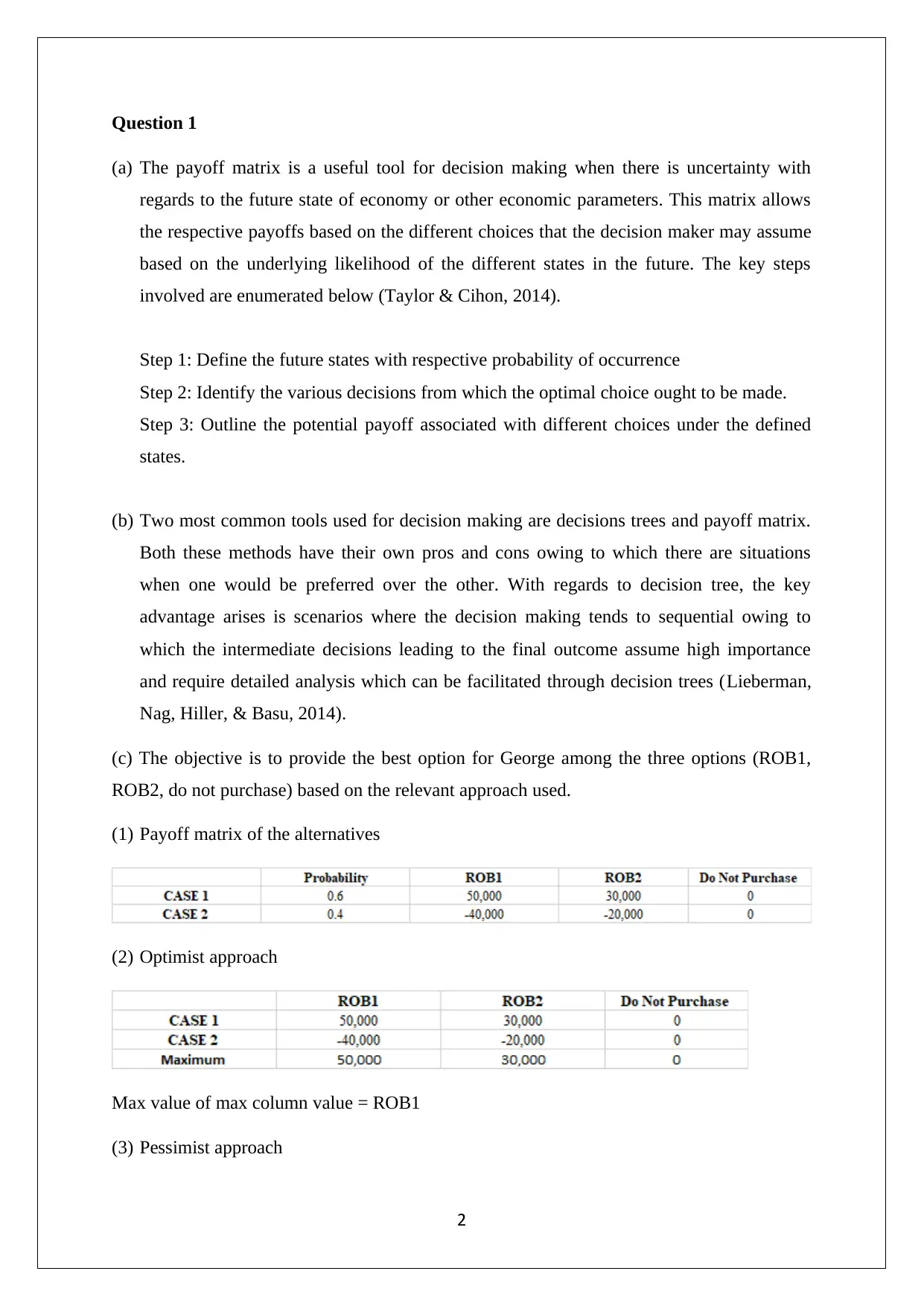
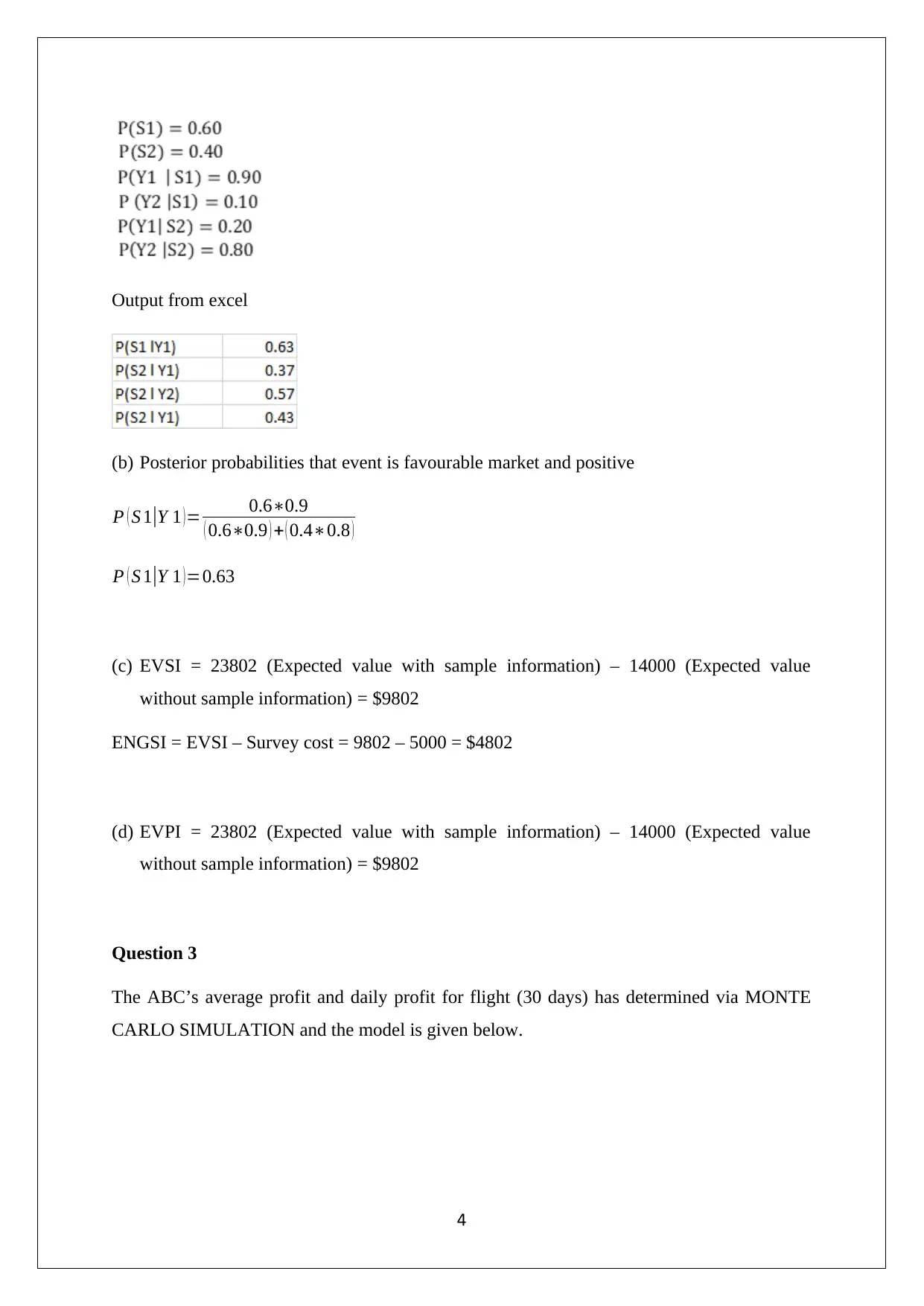
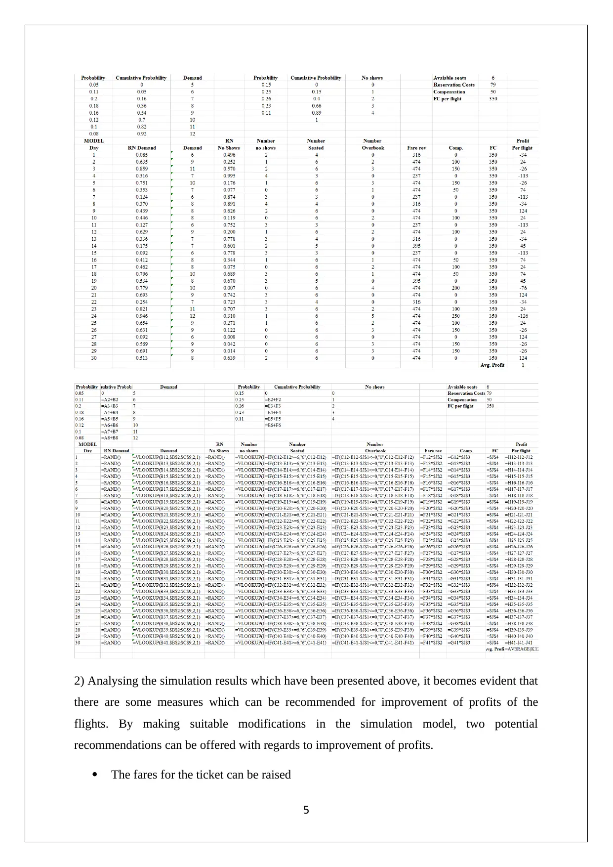
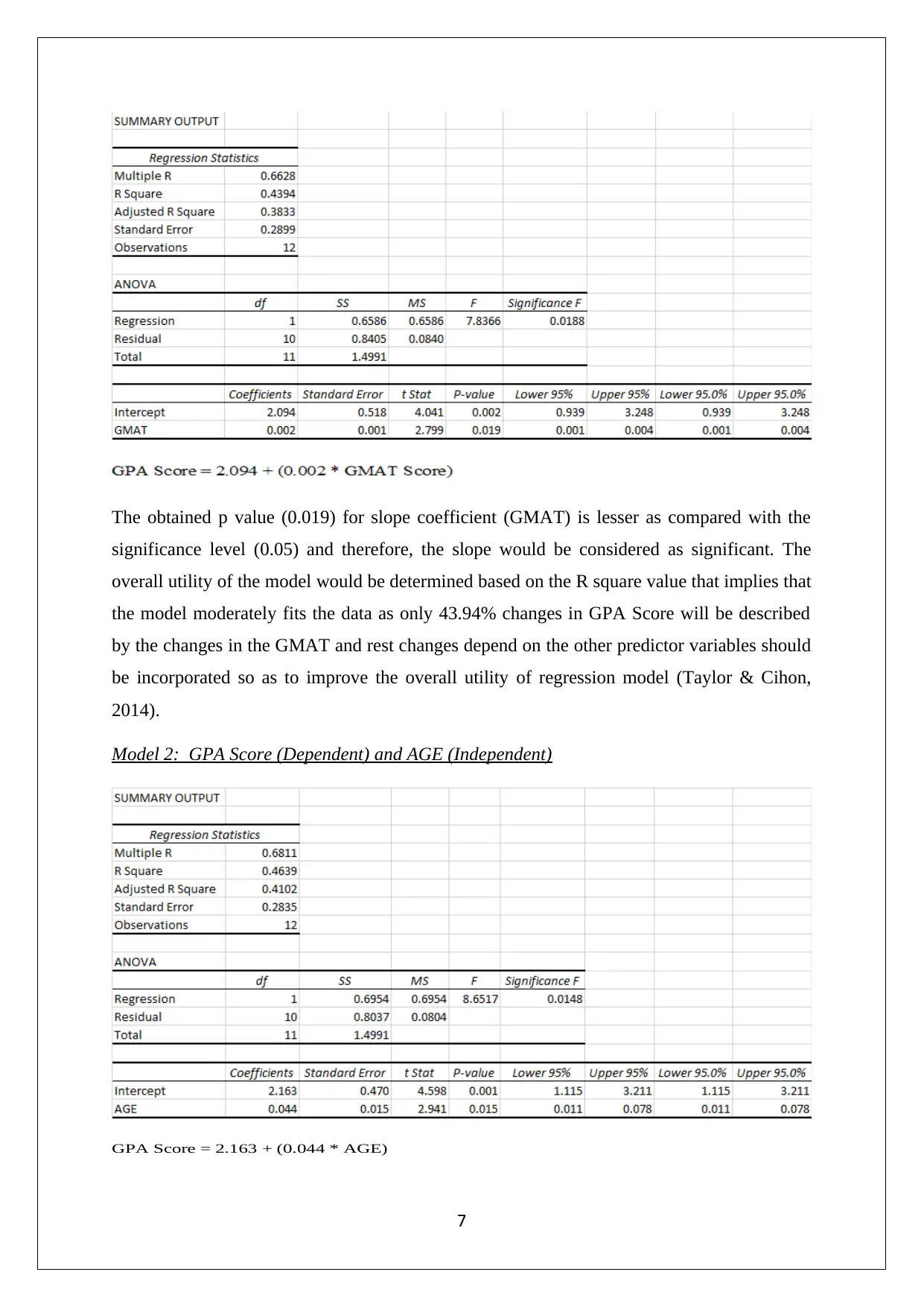
This assignment solution delves into various decision support tools crucial for business development. It begins by explaining the payoff matrix, outlining its steps, and comparing it with decision trees, highlighting their respective advantages. The solution then presents a case study involving George Goleb's robot purchase, employing payoff matrix, and different decision-making approaches like optimist, pessimist, Laplace, criterion of regret, and EMV to determine the best option. The analysis extends to probability calculations, including revised prior probabilities, and posterior probabilities. The solution also includes Expected Value of Sample Information (EVSI) and Expected Value of Perfect Information (EVPI) calculations. Furthermore, the assignment incorporates a Monte Carlo simulation to analyze average and daily flight profits, proposing recommendations for profit improvement. Regression models are developed to analyze GPA scores, and break-even analysis and margin of safety calculations are provided. The solution utilizes formulas and computations to arrive at the final answer with relevant references to support the analysis.

DECISION SUPPORT TOOLS
STUDENT ID:
[Pick the date]

Question 1
(a) The payoff matrix is a useful tool for decision making when there is uncertainty with
regards to the future state of economy or other economic parameters. This matrix allows
the respective payoffs based on the different choices that the decision maker may assume
based on the underlying likelihood of the different states in the future. The key steps
involved are enumerated below (Taylor & Cihon, 2014).
Step 1: Define the future states with respective probability of occurrence
Step 2: Identify the various decisions from which the optimal choice ought to be made.
Step 3: Outline the potential payoff associated with different choices under the defined
states.
(b) Two most common tools used for decision making are decisions trees and payoff matrix.
Both these methods have their own pros and cons owing to which there are situations
when one would be preferred over the other. With regards to decision tree, the key
advantage arises is scenarios where the decision making tends to sequential owing to
which the intermediate decisions leading to the final outcome assume high importance
and require detailed analysis which can be facilitated through decision trees (Lieberman,
Nag, Hiller, & Basu, 2014).
(c) The objective is to provide the best option for George among the three options (ROB1,
ROB2, do not purchase) based on the relevant approach used.
(1) Payoff matrix of the alternatives
(2) Optimist approach
Max value of max column value = ROB1
(3) Pessimist approach
2

Max value of min column value = Do not purchase
(4) Lapalce criterion approach
Max average of average value = Either ROB1 or ROB 2 (both shows same average)
(5) Criterion of regret approach
Minimum value of max row value = ROB2
(6) EMV approach
Max EMV value = ROB 1
Question 2
Notation
(a) Revised prior probabilities
The respective probabilities can be determined as shown below.
3

Output from excel
(b) Posterior probabilities that event is favourable market and positive
P ( S 1|Y 1 )= 0.6∗0.9
( 0.6∗0.9 ) + ( 0.4∗0.8 )
P ( S 1|Y 1 )=0.63
(c) EVSI = 23802 (Expected value with sample information) – 14000 (Expected value
without sample information) = $9802
ENGSI = EVSI – Survey cost = 9802 – 5000 = $4802
(d) EVPI = 23802 (Expected value with sample information) – 14000 (Expected value
without sample information) = $9802
Question 3
The ABC’s average profit and daily profit for flight (30 days) has determined via MONTE
CARLO SIMULATION and the model is given below.
4

2) Analysing the simulation results which have been presented above, it becomes evident that
there are some measures which can be recommended for improvement of profits of the
flights. By making suitable modifications in the simulation model, two potential
recommendations can be offered with regards to improvement of profits.
 The fares for the ticket can be raised
5

 The compensation for the overbooking can be brought down.
In relation to the above recommendations, it is noteworthy that any changes in the above
parameters could also lead to changes in the demand pattern along with the respective
probability of overbooking. Only once these changes have been considered could an
informed decision be taken by the management.
Considering the simulation results that have been obtained, it is apparent that while the
current operations are profitable, certain measures can be undertaken to improve upon the
same. One of these relates to rise in fares especially in the context of robust demand where
overbooking is a common phenomenon. However, currently the company is overbooking
owing to the fact that because of no shows it is able to earn a higher profit. Thereby, any
increase in fare may hamper demand and reduce the extent of overbooking which can have
adverse impact on profit and may limit the upside. This cannot be determined from the given
model as it is based on a given demand and no turn up schedule. A similar problem may arise
in regards to the reduction of overbooking compensation. As a result, the company needs to
analyse these recommendations thoroughly and should roll out only after a small pilot project
in this regards.
Yours Sincerely
STUDENT NAME
Question 4
Regression Models
Model 1: GPA Score (Dependent) and GMAT Score (Independent)
6

The obtained p value (0.019) for slope coefficient (GMAT) is lesser as compared with the
significance level (0.05) and therefore, the slope would be considered as significant. The
overall utility of the model would be determined based on the R square value that implies that
the model moderately fits the data as only 43.94% changes in GPA Score will be described
by the changes in the GMAT and rest changes depend on the other predictor variables should
be incorporated so as to improve the overall utility of regression model (Taylor & Cihon,
2014).
Model 2: GPA Score (Dependent) and AGE (Independent)
GPA Score = 2.163 + (0.044 * AGE)
7

The obtained p value (0.015) for slope coefficient (AGE) is lesser as compared with the
significance level (0.05) and therefore, the slope would be considered as significant. The
overall utility of the model would be determined based on the R square value that implies that
the model moderately fits the data as only 46.39% changes in GPA Score will be described
by the changes in the AGE and rest changes depend on the other predictor variables should be
incorporated so as to improve the overall utility of regression model (Shi & Tao, 2015).
Model 3: GPA Score (Dependent) and GMAT Score & AGE (Independent)
GPA Score = 1.378 + (0.002 * GMAT Score) + (0.034 *AGE)
The obtained p values for slope coefficients (GMAT and AGE) is lesser as compared with the
significance level (0.05) and therefore, the slopes would be considered as significant. The
overall utility of the model would be determined based on the R square value that implies that
the model moderately strong fits the data as only 69.45% changes in GPA Score will be
described by the changes in the GMAT and AGE (Medhi, 2016).
(2) R Square also known as coefficient of determination. This is the decision variable to
select the most appropriate regression model for analysis. The regression model that has
maximum R square value would be termed as most suitable regression model owing to the
predictive power being the highest (Hillier, 2016).
8

It is apparent from the above that regression model 3 has maximum R square value and
hence, the best model would be model 3 i.e. multiple regression model.
(3) Computation of the GPA score for the given inputs
Question 5
(a) Calculation for break-even number of units and dollars
Contribution margin per unit of product A
= Per unit selling price – Per unit variable cost = $12-$6 = $6
Break even number of units
= Fixed cost of product A / Contribution margin per unit of product A
= 1200 / 6 = 200
Break even number of dollars
= Break even number of units * Per unit selling price
= 200 * 12 = $24,000
(b) Calculation of number of units and margin of safety
Number of units
9

= (Fixed cost of product A + Target profit) / Contribution margin per unit of product A
= (1200 +600) / 6 = 300
Margin of safety
= (Number of units * Per unit selling price) – Per unit selling price (Fixed cost of product
A /Contribution margin per unit of product A)
= (300 * 12) – 12*(1200/6) = $1200
(c) Units of product A is 2 X and of product B is X.
Contribution margin per unit of product B
= Per unit selling price – Per unit variable cost = $20-$8 = $12
Profit prior to tax
= Post tax profit / (1- tax rate) = 1400/ (1- 30%) = $2000
Gross profit generated for product A and B
=Unit contribution margin of product A * Units of A = 6* 2 X = 12 X
= Unit contribution margin of product B * Units of A = 12* X = 12 X
Gross profit of both products = 24 X
Fixed cost = Gross profit of both products – Profit prior to tax
5200 = 24X – 2000
X = 300
Therefore,
Units of A = 2X = 600
In dollars = Units * Per unit selling price = 600 * 12 = $3,600
Units of B = X = 300
In dollars = Units * Per unit selling price = 300 * 20 = $6000
10

References
Hillier, F. (2016).Introduction to Operations Research.(6thed.). New York: McGraw Hill
Publications.
Lieberman, F. J., Nag, B., Hiller, F.S. & Basu, P. (2014).Introduction To Operations
Research (5thed.).New Delhi: Tata McGraw Hill Publishers.
Medhi, J. (2016). Statistical Methods: An Introductory Text (4thed.). Sydney: New Age
International.
Shi, Z. N. & Tao, J. (2015).Statistical Hypothesis Testing: Theory and Methods (6thed.).
London: World Scientific.
Taylor, K. J. & Cihon, C. (2014).Statistical Techniques for Data Analysis (2nded.).
Melbourne: CRC Press.
11