Decision Support Tools in Business: Analysis, Simulations, and Models

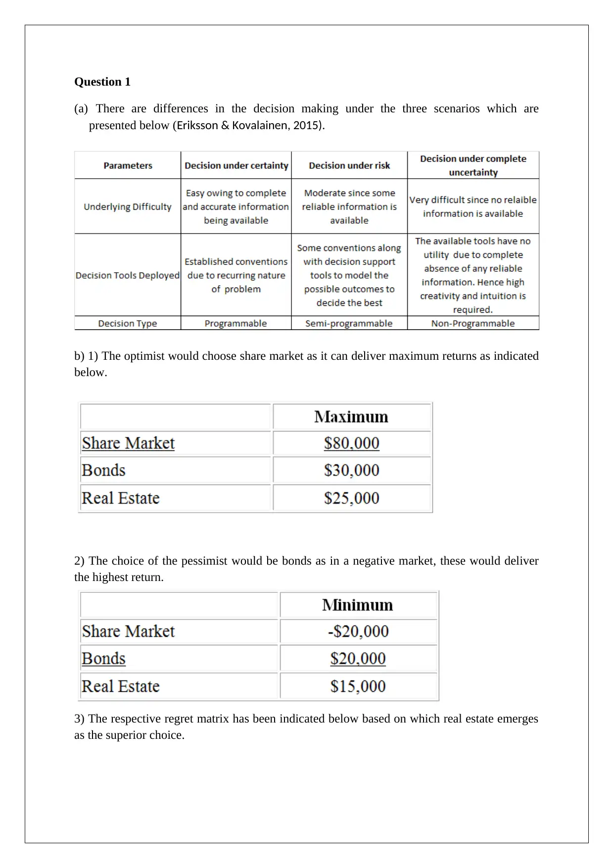
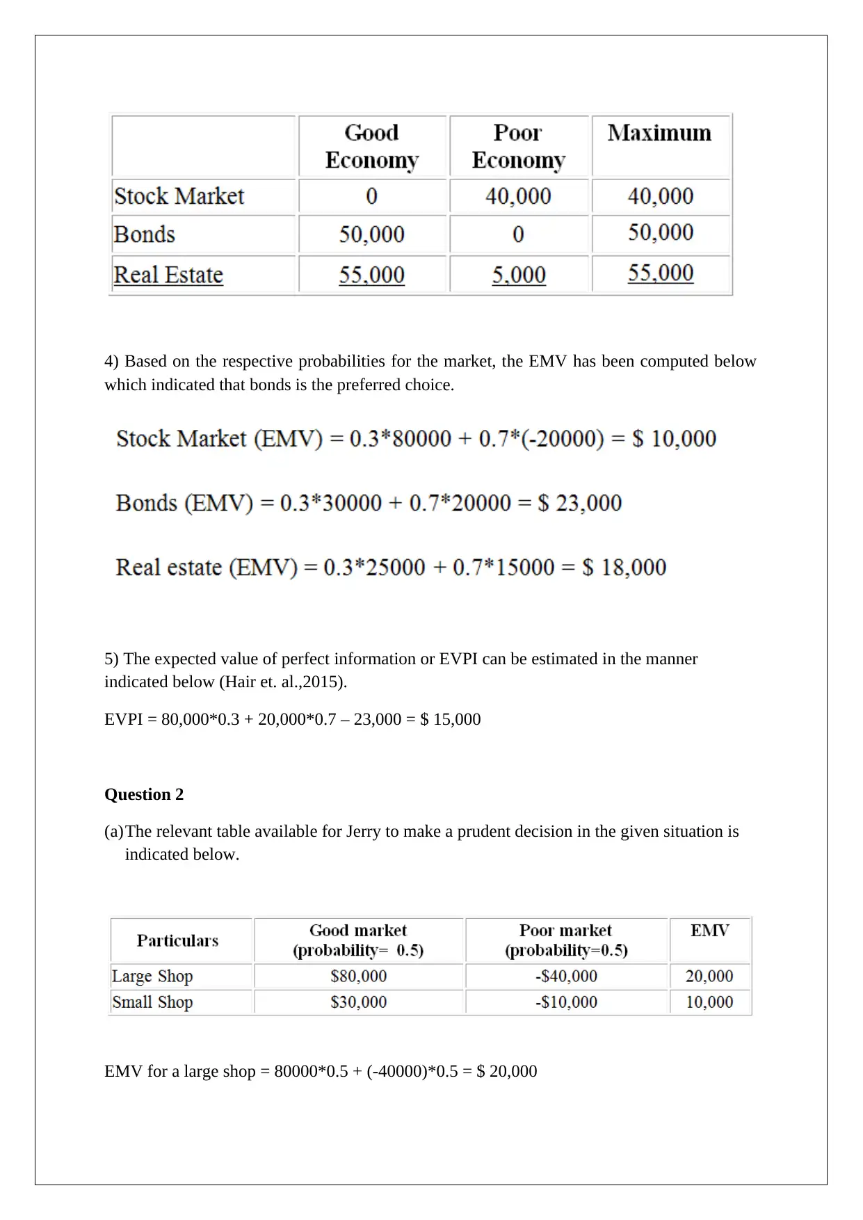
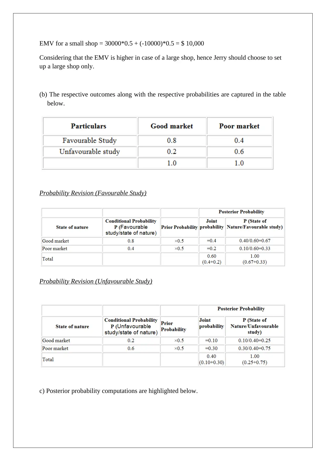
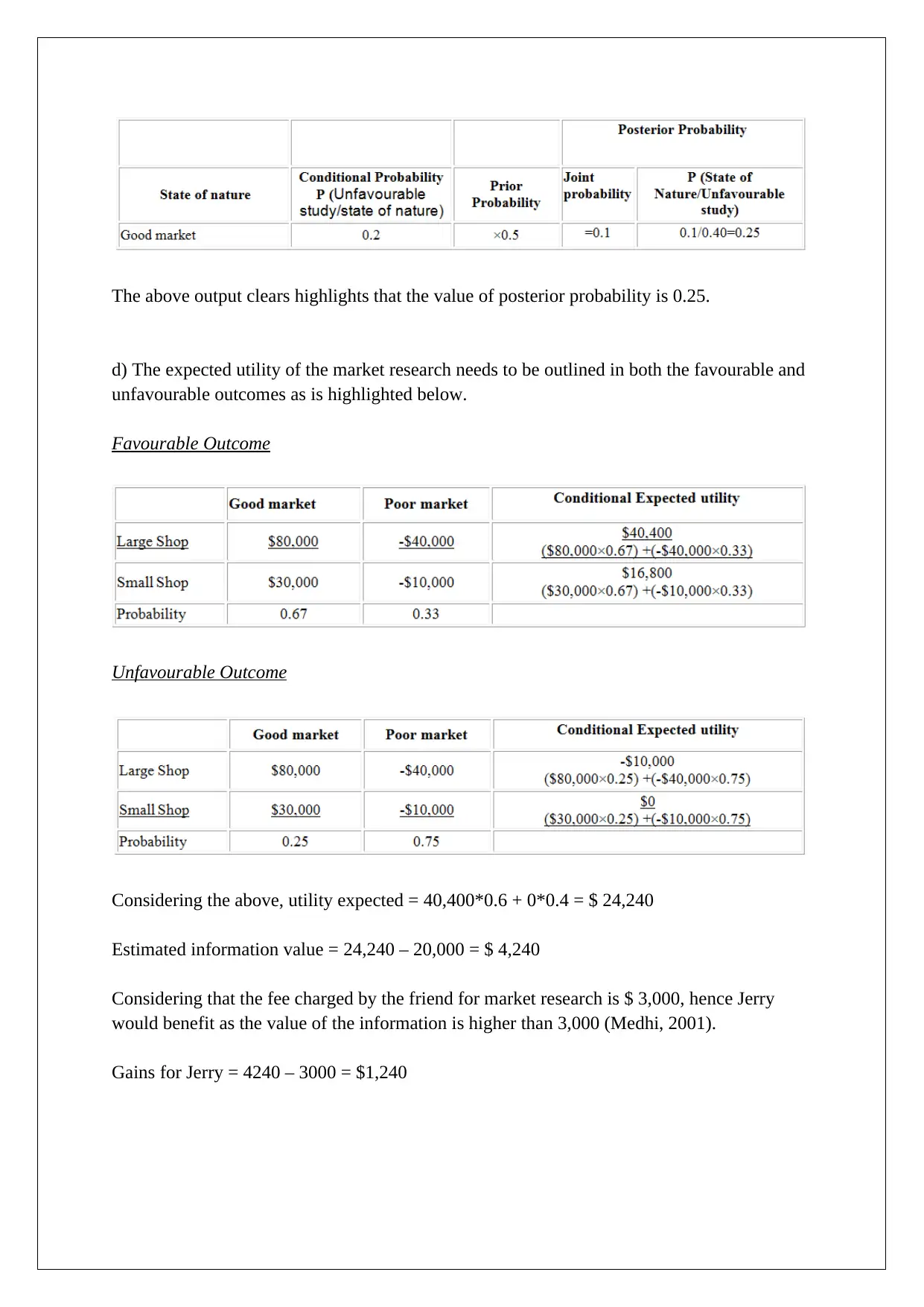
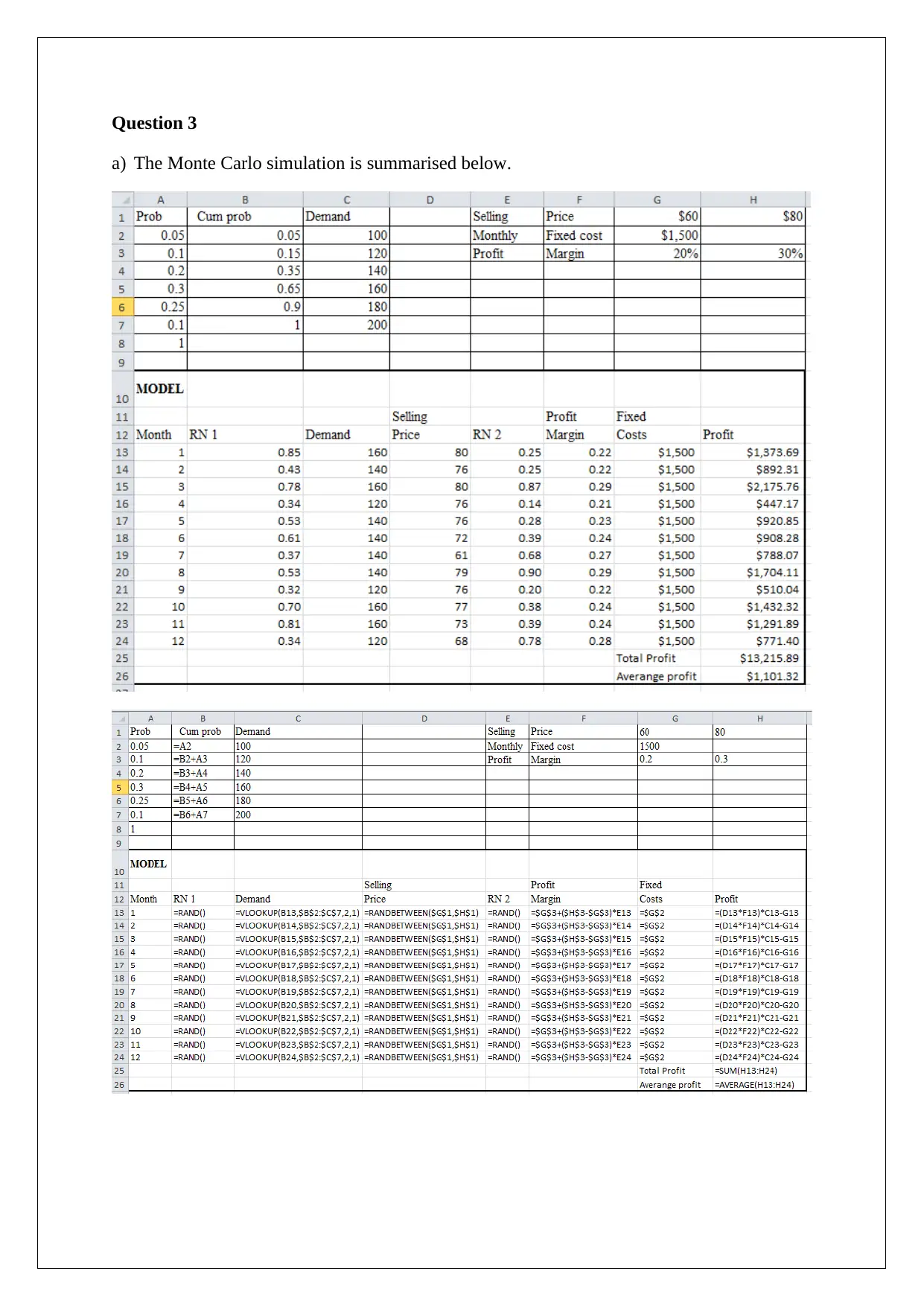
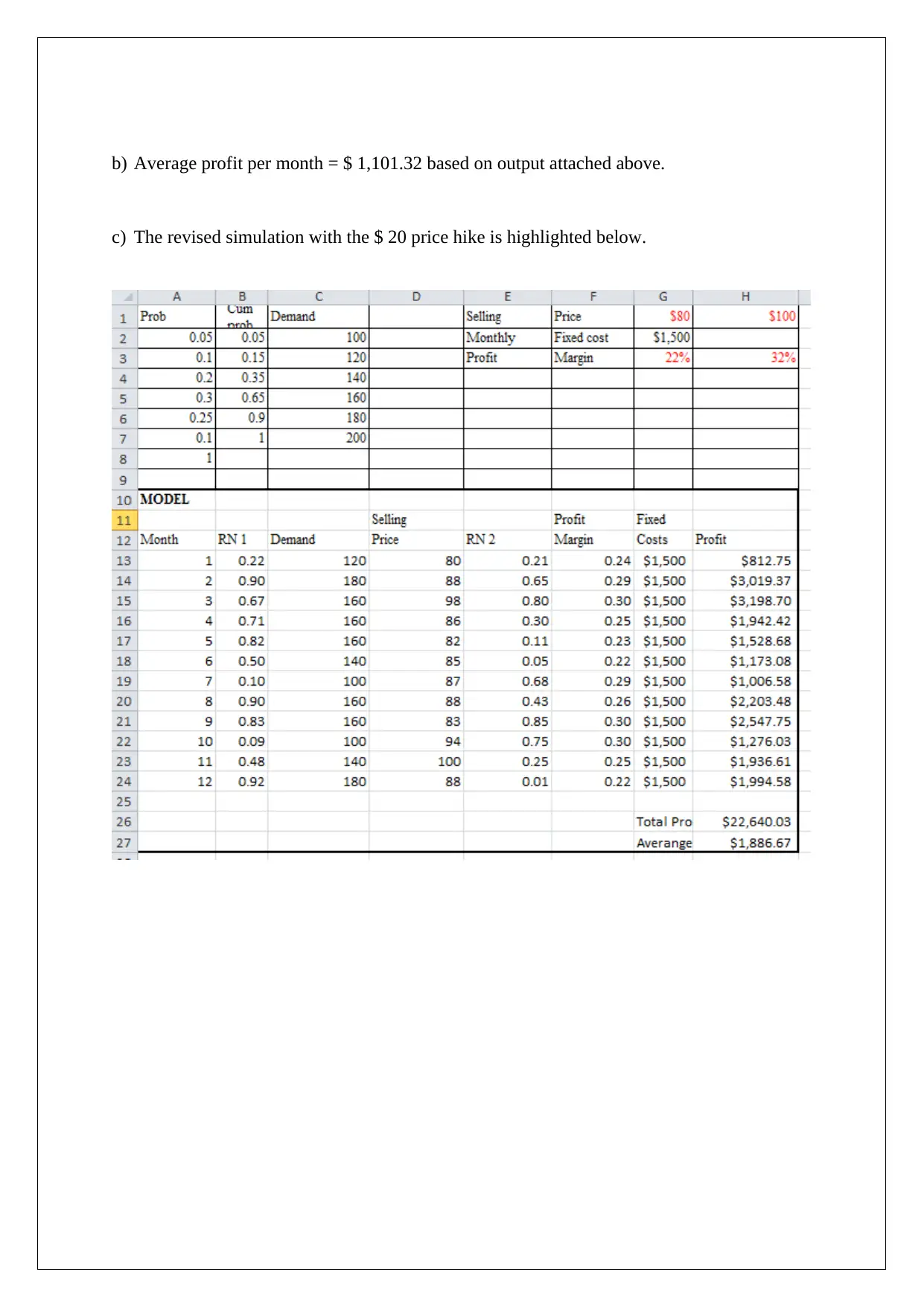
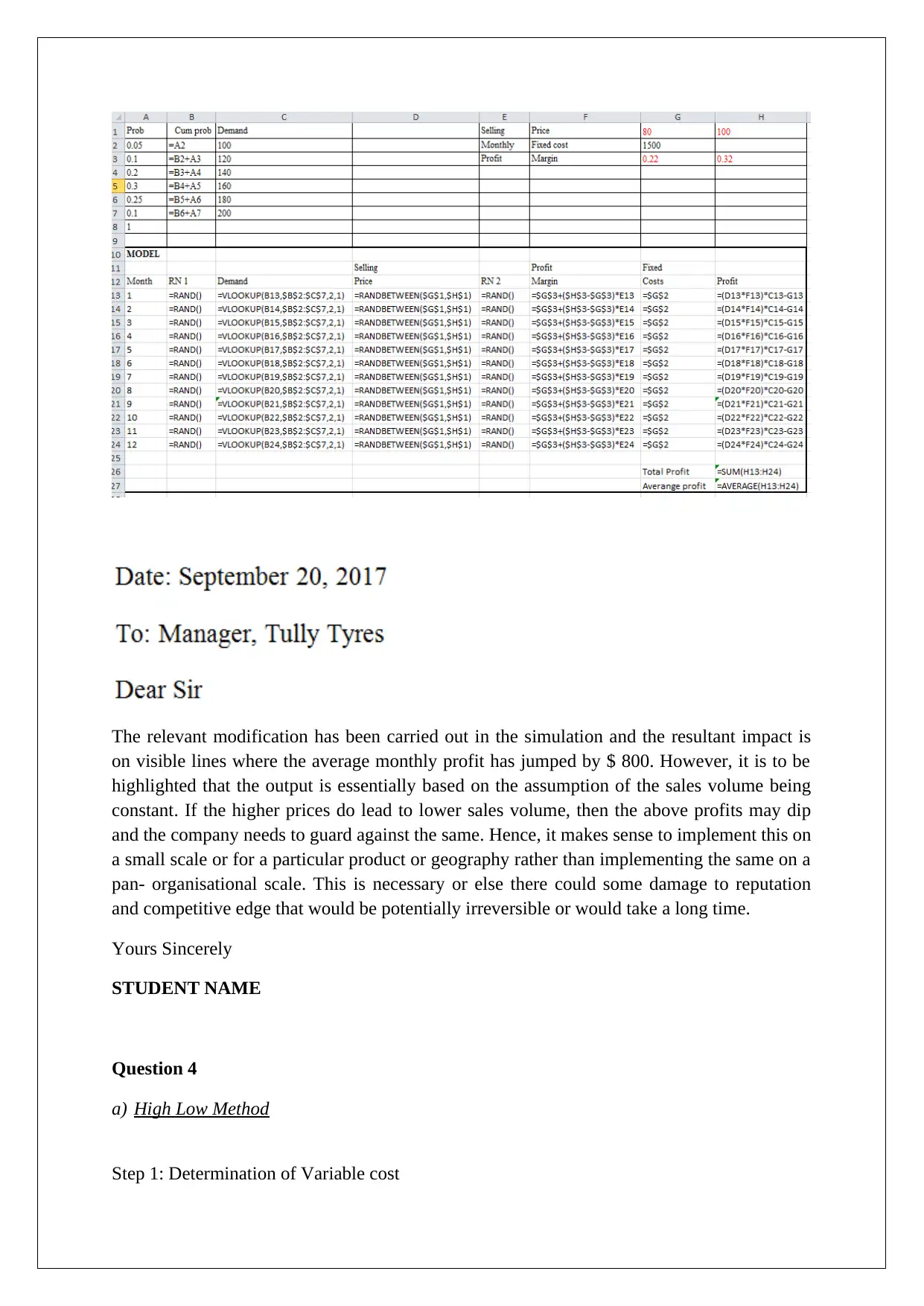
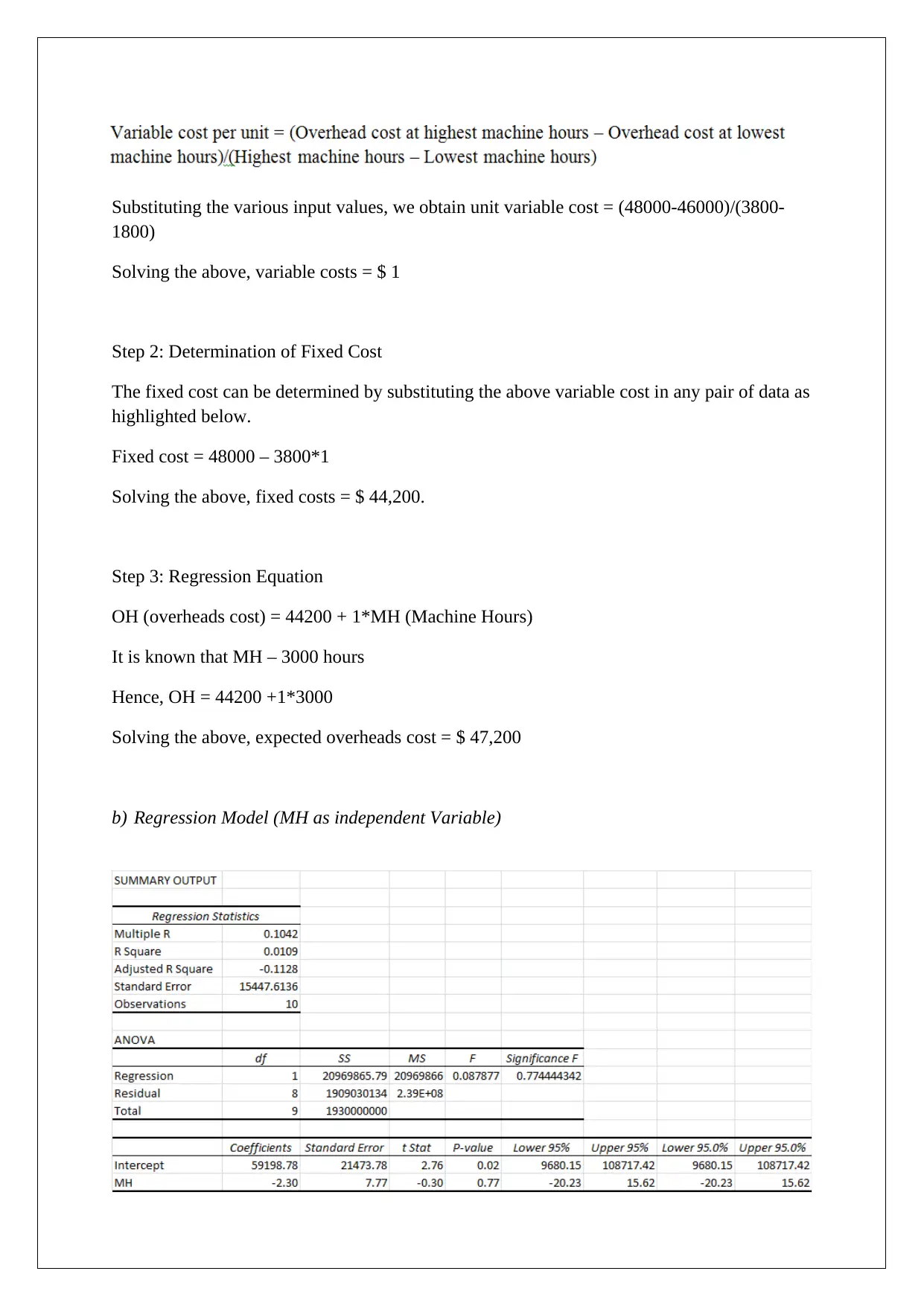
This assignment solution addresses several key concepts in decision support tools. It begins with a comparison of decision-making under different scenarios, including the application of EMV, regret matrices, and EVPI. The solution then analyzes a scenario involving market research and posterior probabilities to determine the optimal business decision. Following this, the assignment explores Monte Carlo simulation to assess the impact of price changes on profit and provides a detailed explanation of the high-low method and regression analysis, using different variables to estimate overhead costs. Finally, the solution concludes with break-even analysis for two products, considering different sales ratios and profit targets, and determining the sales volumes required to achieve specific pre- and post-tax profit levels. The assignment uses various statistical techniques and financial models to support business decision-making.

DECISION SUPPORT TOOLS
STUDENT ID:
[Pick the date]

Question 1
(a) There are differences in the decision making under the three scenarios which are
presented below (Eriksson & Kovalainen, 2015).
b) 1) The optimist would choose share market as it can deliver maximum returns as indicated
below.
2) The choice of the pessimist would be bonds as in a negative market, these would deliver
the highest return.
3) The respective regret matrix has been indicated below based on which real estate emerges
as the superior choice.

4) Based on the respective probabilities for the market, the EMV has been computed below
which indicated that bonds is the preferred choice.
5) The expected value of perfect information or EVPI can be estimated in the manner
indicated below (Hair et. al.,2015).
EVPI = 80,000*0.3 + 20,000*0.7 – 23,000 = $ 15,000
Question 2
(a)The relevant table available for Jerry to make a prudent decision in the given situation is
indicated below.
EMV for a large shop = 80000*0.5 + (-40000)*0.5 = $ 20,000

EMV for a small shop = 30000*0.5 + (-10000)*0.5 = $ 10,000
Considering that the EMV is higher in case of a large shop, hence Jerry should choose to set
up a large shop only.
(b) The respective outcomes along with the respective probabilities are captured in the table
below.
Probability Revision (Favourable Study)
Probability Revision (Unfavourable Study)
c) Posterior probability computations are highlighted below.

The above output clears highlights that the value of posterior probability is 0.25.
d) The expected utility of the market research needs to be outlined in both the favourable and
unfavourable outcomes as is highlighted below.
Favourable Outcome
Unfavourable Outcome
Considering the above, utility expected = 40,400*0.6 + 0*0.4 = $ 24,240
Estimated information value = 24,240 – 20,000 = $ 4,240
Considering that the fee charged by the friend for market research is $ 3,000, hence Jerry
would benefit as the value of the information is higher than 3,000 (Medhi, 2001).
Gains for Jerry = 4240 – 3000 = $1,240

Question 3
a) The Monte Carlo simulation is summarised below.

b) Average profit per month = $ 1,101.32 based on output attached above.
c) The revised simulation with the $ 20 price hike is highlighted below.

The relevant modification has been carried out in the simulation and the resultant impact is
on visible lines where the average monthly profit has jumped by $ 800. However, it is to be
highlighted that the output is essentially based on the assumption of the sales volume being
constant. If the higher prices do lead to lower sales volume, then the above profits may dip
and the company needs to guard against the same. Hence, it makes sense to implement this on
a small scale or for a particular product or geography rather than implementing the same on a
pan- organisational scale. This is necessary or else there could some damage to reputation
and competitive edge that would be potentially irreversible or would take a long time.
Yours Sincerely
STUDENT NAME
Question 4
a) High Low Method
Step 1: Determination of Variable cost

Substituting the various input values, we obtain unit variable cost = (48000-46000)/(3800-
1800)
Solving the above, variable costs = $ 1
Step 2: Determination of Fixed Cost
The fixed cost can be determined by substituting the above variable cost in any pair of data as
highlighted below.
Fixed cost = 48000 – 3800*1
Solving the above, fixed costs = $ 44,200.
Step 3: Regression Equation
OH (overheads cost) = 44200 + 1*MH (Machine Hours)
It is known that MH – 3000 hours
Hence, OH = 44200 +1*3000
Solving the above, expected overheads cost = $ 47,200
b) Regression Model (MH as independent Variable)

The simple regression equation is as indicated follows..
OH = 59198.78 – 2.30*MH
Comment:
Ho: βMH = 0
Hi: βMH ≠ 0
The relevant t stat = -0.30 and corresponding p value = 0.77
Since p> significance level, null hypothesis cannot be rejected and hence slope is
insignificant.
Also, the R-square value is abysmally low which combined with the insignificant slope
reflects the model being a poor fit (Halhn & Doganaksoy, 2011).
Regression Model (Batches as independent variable)
The simple regression equation is as indicated follows.
OH = 6555.56 + 234.57* Batches
Comment:
Ho: βbatches = 0
Hi: βbatches ≠ 0
The relevant t stat = 6.28 and corresponding p value = 0.00
Since p< significance level, null hypothesis can be rejected and hence slope is significant.

Also, the R-square value is quite high which combined with the significant slope reflects the
model being a good fit.
Multiple Regression Model ( Batches and machine hours as independent variables)
The linear regression equation is as indicated follows.
OH = 9205.66 -0.93*MH+233.83*Batches
Comment:
Ho: βbatches = 0
Hi: βbatches ≠ 0
The relevant t stat = 5.87 and corresponding p value = 0.00
Since p< significance level, null hypothesis can be rejected and hence slope is significant.
Ho: βMH = 0
Hi: βMH ≠ 0
The relevant t stat = -0.27 and corresponding p value = 0.79
Since p> significance level, null hypothesis cannot be rejected and hence slope is
insignificant.
Also, the R-square value is quite high which combined with the significant slope reflects the
model being a good fit (Holsapple & Whinston, 2013).

c) The various pivotal factors are outlined below (Lind, Marchal & Wathen, 2012).
 R2 – The highest value is observed for multiple regression model but it can be on
account of an incremental predictor, hence adjusted R2 is preferable.
 Adjusted R2 – The highest value is observed for linear regression model
(Independent Variable: Batches).
 ANOVA output – The corresponding F statistic from regression ANOVA outputs
is maximum in case of linear regression model (Independent Variable: Batches).
Hence, the best regression model to be selected would be linear regression model
(Independent Variable: Batches).
d) The best regression model has the following equation.
OH =6555.56 +234.57*Batches
The given input for batches is given as 150. Substituting the same, we get,
OH = 6555.56 + 234.57*150
Solving the above, OH = $ 41,740.74
Question 5
(a) Product A (Contribution margin per unit) = 10 – 5 = $ 5
Product B (Contribution margin per unit) = 20-12 = $ 8
(b) Total fixed costs (given) = $ 4000
Product B (Contribution margin per unit) = $ 8
Hence, unit break even = (4000/8) or 500 units
(c)Total fixed costs (given) = $ 4000
Product A (Contribution margin per unit) = $ 5
Hence, unit break even = (4000/5) or 800 units
Sales volume for breakeven = Price *Breakeven Units = 10*800 = $ 8,000

(d)The two products are sold maintaining a ratio of 2:1 in favour of product A.
(i) The contribution margin on an average basis = (2/3)*5 + (1/3)*8 = $ 6
The objective is to obtain a pre-tax profit of $ 5,000
Sales volume = (Pre-tax profit + Fixed cost)/Contribution margin(average) = (5000+4000)/6
Solving the above, we get sales volume = 1500 units
Dividing the above in 2:1 ratio, product A would have sales of 1000 units while product B
would have sales of 500 units.
(ii) The post-tax profit that the company wants to achieve is $ 21,000
Equivalent pre-tax profit = 21000/0.7 or $ 30,000
Sales volume = (Pre-tax profit + Fixed cost)/Contribution margin(average) = (30000+4000)/6
Solving the above, we get sales volume = 5667 units
Dividing the above in 2:1 ratio, product A would have sales of 3778 units while product B
would have sales of 1889 units.
References

Eriksson, P. & Kovalainen, A. (2015). Quantitative methods in business research (3rd ed.).
London: Sage Publications.
Hair, J. F., Wolfinbarger, M., Money, A. H., Samouel, P., & Page, M. J. (2015). Essentials of
business research methods (2nd ed.). New York: Routledge.
Halhn, J. G. & Doganaksoy, N. (2011) The Role of Statistics in Business and Industry (7th ed.).
London: London: John Wiley.
Holsapple, C. & Whinston, B.A. (2013) Decision Support Systems: Theory and Application (6th
ed.). Sydney: Springer Science & Business Media.
Lind, A.D., Marchal, G.W. & Wathen, A.S. (2012). Statistical Techniques in Business and
Economics (15th ed.). New York : McGraw-Hill/Irwin.
Medhi, J. (2001). Statistical Methods: An Introductory Text (4th ed.). Sydney: New Age
International.