PACC6008 - Statistical Analysis in Business Decision Making

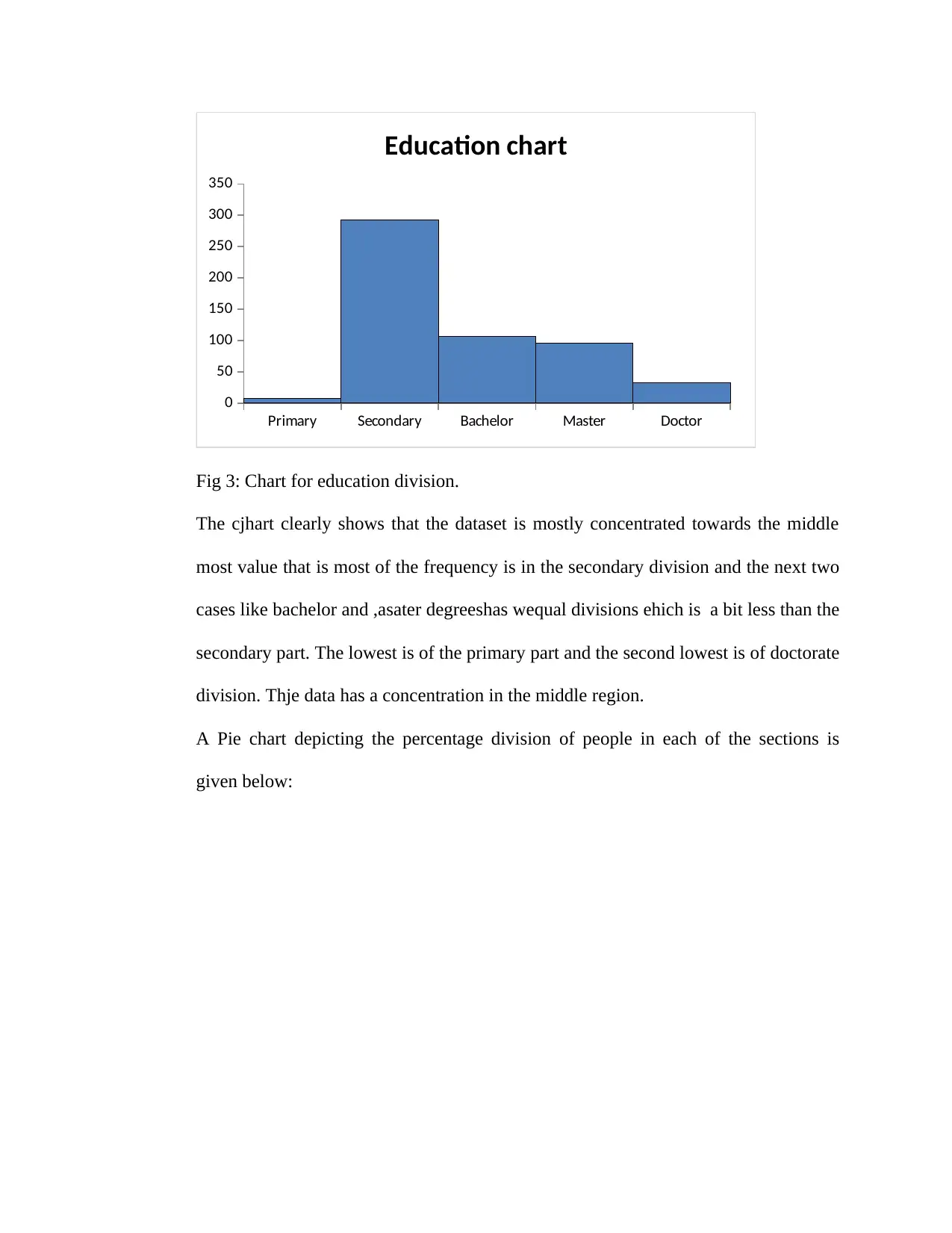
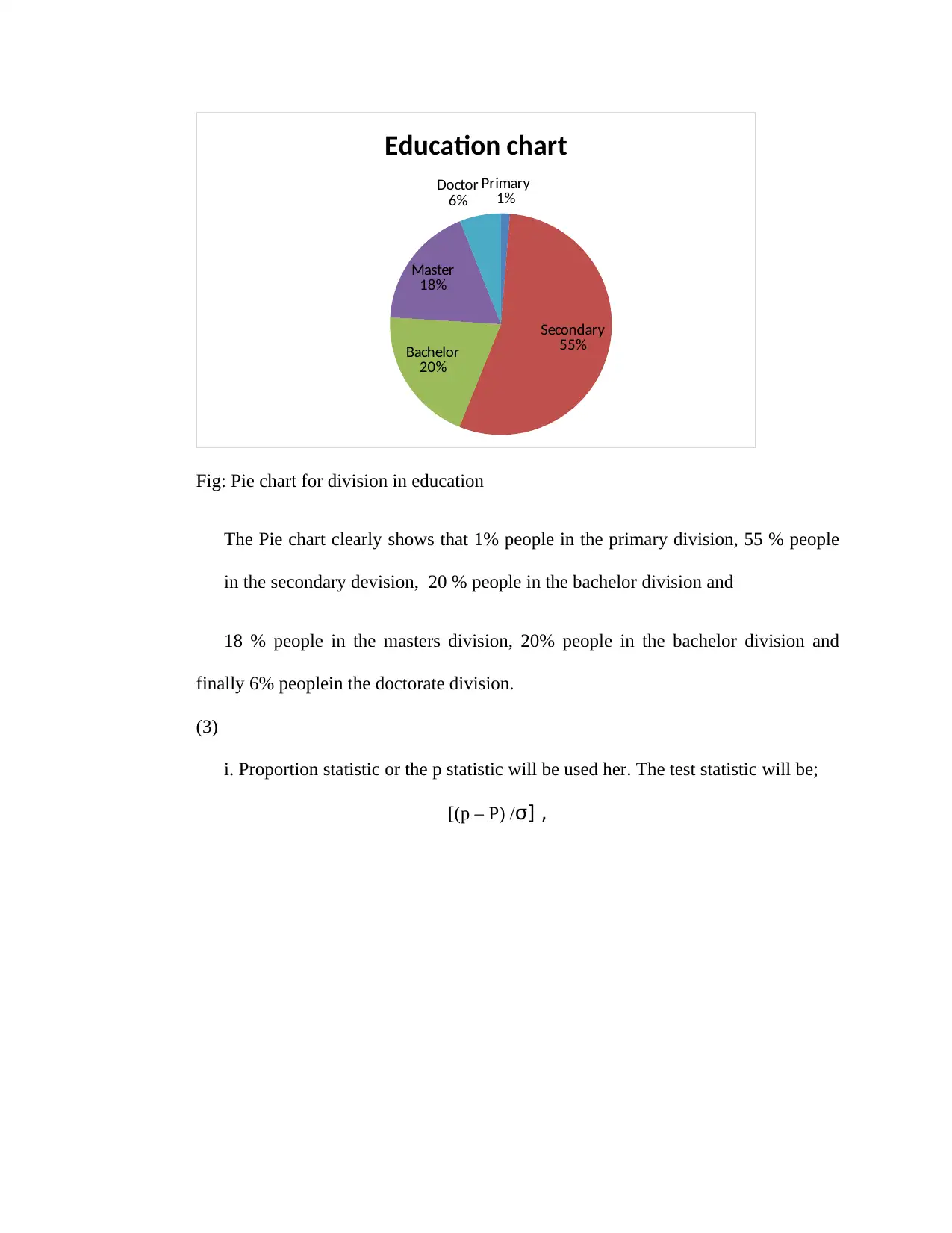
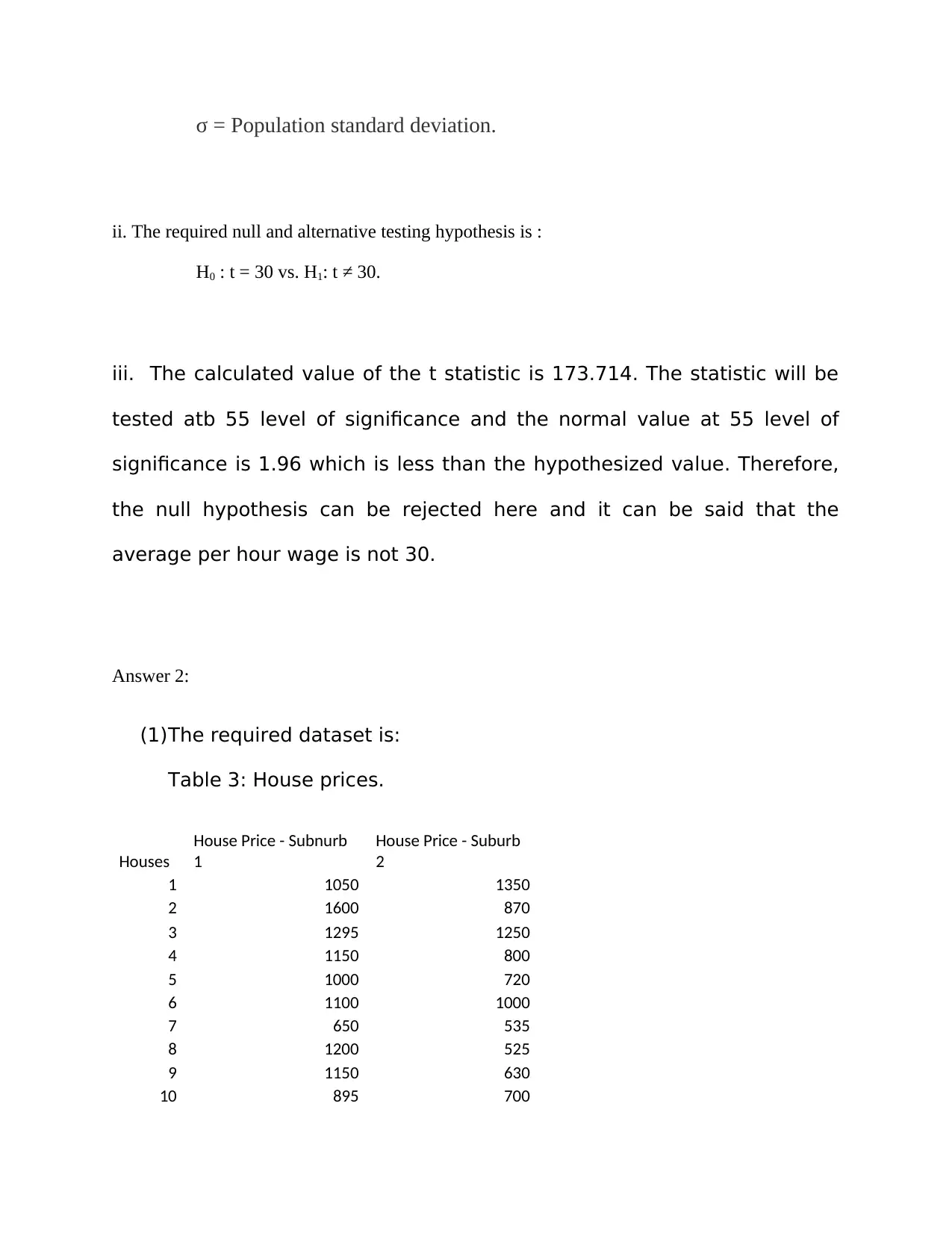
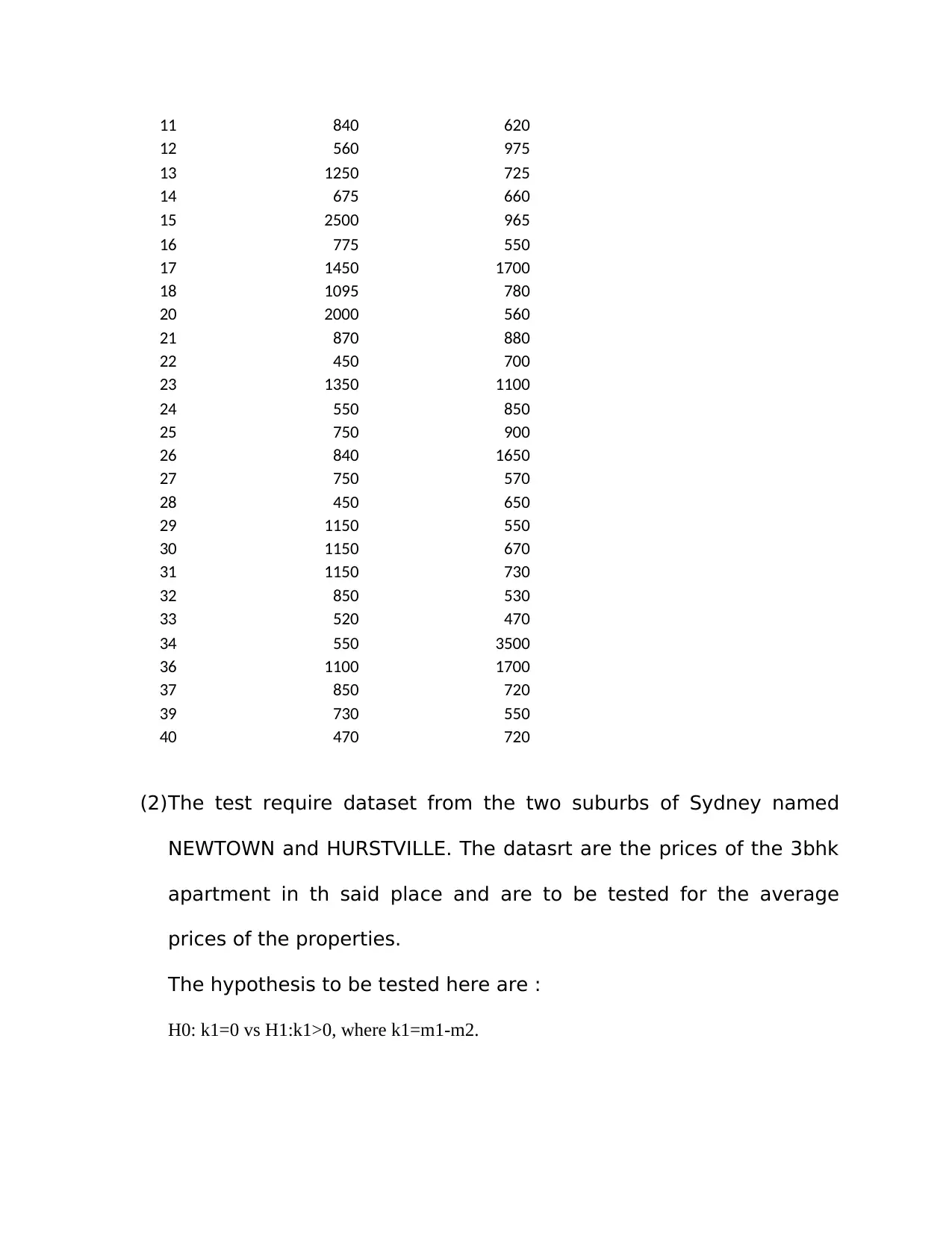
This assignment focuses on statistical analysis for business decision-making. It includes descriptive statistical analysis of wages and education levels, using histograms and pie charts to visualize data distribution. Hypothesis testing is conducted to determine if the proportion of tertiary education has increased and whether the average hourly wage is a specific value. A t-test is performed to compare average house prices in two suburbs, Newtown and Hurstville, to assess if there is a significant difference. The assignment uses statistical tools to analyze provided datasets and draw conclusions based on the test results, providing a comprehensive approach to quantitative research in a business context. Desklib provides a range of solved assignments and past papers for students.

BUSINESS DECISION MAKING
Name of the student:
Name of the university:
Author’s note:

Answer 1:
 Population Web institute is interested in checking about the Education qualification
division and wage division among people of the said region. It can be said that their
is a connection between the two variables and it can be tested here.
 For Wages:
Given is the data set for wages. A descriptive statiscal analysis report of the given
variable is given below:
Table 1: Descriptive analysis of wages.
Mean 25.61666667
Standard Error 0.340206957
Median 23.75
Mode 25
Standard
Deviation 7.86165206
Sample Variance 61.80557311
Kurtosis 4.807383971
Skewness 1.57737306
Range 60
Minimum 10
Maximum 70
Sum 13679.3
Count 534
1st Quartile 21.25
3rd Quartile 28
IQR 6.75
It can be said from the table that the average wage of people in the said are ais
25.616667 and it can vary within a range of 0.3402. Maximum people has the wage
of 25 and 25 % people has wage above 28 and 25 % has wages below 21.25 and 50%
people have wages in the range of 21.25 and 28. Again, 50% has wages below 23.75
and 50% has wages above 23.75. The maximum wage is 70 and the minimum wage is
10.

A histogram can be posted here depicting distribution of wages.
20-Oct 20-30 30-40 40-50 50-60 60-70
0
50
100
150
200
250
300
350
400
Wage chart
Fig 1: Histogram for wages.
It can be said from the histogram that the variable wage has a distribution towards the
low wages category. Therefore, the distribution is left tailed.
A Pie chart depicting the percentage of people in the different wage group is attached
below.
20-Oct
16%
20-30
65%
30-40
15%
40-50
4%
50-60
1% 60-70
0%
Wage chart
Fig 2: Pie chart for wages.

The Pie chart shows percentage of people in the different divisions. The division of
10-20 has 16% of people, the division of 20-30 has 64% of people which is the
highest one, the division of 30-40 has 15% of people, the division of 40-50 has 4% of
people, the division of 50-60 has 1 %of people and the last division of 60-70 has 0%
of people.
For Education:
A descriptive statistical test depicting data features here can be shown here.
Table 2: Descriptive analysis for Education.
Mean 2.726078799
Standard Error 0.042159852
Median 2
Mode 2
Standard
Deviation 0.973335773
Sample Variance 0.947382528
Kurtosis
-
0.364587077
Skewness 0.878054936
Range 4
Minimum 1
Maximum 5
Sum 1453
Count 533
The maximum frequency is of 2 that is people with secondary education and there are
533 people in total.
A histogram depicting the distribution of this education division is geiven below:

Primary Secondary Bachelor Master Doctor
0
50
100
150
200
250
300
350
Education chart
Fig 3: Chart for education division.
The cjhart clearly shows that the dataset is mostly concentrated towards the middle
most value that is most of the frequency is in the secondary division and the next two
cases like bachelor and ,asater degreeshas wequal divisions ehich is a bit less than the
secondary part. The lowest is of the primary part and the second lowest is of doctorate
division. Thje data has a concentration in the middle region.
A Pie chart depicting the percentage division of people in each of the sections is
given below:

Primary
1%
Secondary
55%Bachelor
20%
Master
18%
Doctor
6%
Education chart
Fig: Pie chart for division in education
The Pie chart clearly shows that 1% people in the primary division, 55 % people
in the secondary devision, 20 % people in the bachelor division and
18 % people in the masters division, 20% people in the bachelor division and
finally 6% peoplein the doctorate division.
(3)
i. Proportion statistic or the p statistic will be used her. The test statistic will be;
[(p – P) /σ] ,

where, p =is the hypothesized value of the statistic,
P = calculated value of the statistic,
ii. The required null and alternative hypothesis for the test is :
H0: p = 0.45 vs. H1: p> 0.45.
iii. Primary and secondary education can be considered here as
tertiary education. There are in total 299 people in the said
group. Therefore, proportion of people in the said group is 0.56,
which is the required calculated proportion. Therefore, the value
of the test statistic will be 5.11.
The statistic is to tested at 5% level of significance. Therefore,
the test significant value is 1.96, which is less than the test
statistic value. Therefore, the null hypothesis can be rejected
here and it can be concluded that the proportion of tertiary
education has increased.
(4)
i. Mean test statistic or the t- statistic will be used her. The
required test statistic is:
t = (M – m)/ σ/√n
where,
m =is the hypothesized value of the statistic,
M = calculated value of the statistic,
n = Total number of observation

σ = Population standard deviation.
ii. The required null and alternative testing hypothesis is :
H0 : t = 30 vs. H1: t ≠ 30.
iii. The calculated value of the t statistic is 173.714. The statistic will be
tested atb 55 level of significance and the normal value at 55 level of
significance is 1.96 which is less than the hypothesized value. Therefore,
the null hypothesis can be rejected here and it can be said that the
average per hour wage is not 30.
Answer 2:
(1)The required dataset is:
Table 3: House prices.
Houses
House Price - Subnurb
1
House Price - Suburb
2
1 1050 1350
2 1600 870
3 1295 1250
4 1150 800
5 1000 720
6 1100 1000
7 650 535
8 1200 525
9 1150 630
10 895 700

11 840 620
12 560 975
13 1250 725
14 675 660
15 2500 965
16 775 550
17 1450 1700
18 1095 780
20 2000 560
21 870 880
22 450 700
23 1350 1100
24 550 850
25 750 900
26 840 1650
27 750 570
28 450 650
29 1150 550
30 1150 670
31 1150 730
32 850 530
33 520 470
34 550 3500
36 1100 1700
37 850 720
39 730 550
40 470 720
(2)The test require dataset from the two suburbs of Sydney named
NEWTOWN and HURSTVILLE. The datasrt are the prices of the 3bhk
apartment in th said place and are to be tested for the average
prices of the properties.
The hypothesis to be tested here are :
H0: k1=0 vs H1:k1>0, where k1=m1-m2.

where, m1 = mean of suburb 1 and
m2 = mean of the suburb 2.
It can be seen from the table here that the t-statistic value is 0.648 and the 2 tailed t significant
value is 1.96. Therefore, the significant value is greater than the statistical value and the null
hypothesis can be accepted here and it can be said that the average prices are equal in both the
regions. Therefore, the test result is that the average prices are equal in both the regions.