Business Dynamics and Problem Solving: A Comprehensive Report

This report delves into the complexities of business dynamics and problem-solving, offering a comprehensive analysis of various methodologies and techniques. The report begins by examining the advantages and disadvantages of business dynamics, emphasizing the use of causal loop diagrams (CLDs) to analyze interrelationships between variables. It further explores the development and application of Excel models for simulating business dynamics, focusing on feedback loop models to address business problems such as increasing costs. The report then investigates the roles of supply chain and inventory management, including the use of economic order quantity (EOQ) and production quantity models to optimize costs. Part 2 of the report focuses on a case study of glass manufacturing, using causal loop diagrams to identify the causes and relationships between linked variables. It analyzes the polarity of causal links, providing calculations for each variable, and explores the production ratio parameter. The report highlights the importance of effective inventory management, supply chain optimization, and the use of analytical tools to improve business performance and solve identified problems.

BUSINESS DYNAMICS AND
PROBLEM SOLVING

Table of Contents
INTRODUCTION...........................................................................................................................1
ECA PART 1...................................................................................................................................1
1 (a). Advantage and disadvantage of business dynamics..........................................................1
1 (b). Development and use of Excel models to simulate business dynamics............................1
2 (a). Role of supply chain and inventory management..............................................................2
2 (b). Use of economic order quantity model and production quantity model...........................3
ECA PART 2...................................................................................................................................3
Cause and relationship between linked variables........................................................................3
Polarity of causal link..................................................................................................................4
Calculations for each variable.....................................................................................................6
Production ratio VI parameter.....................................................................................................7
CONCLUSION................................................................................................................................8
REFERENCES................................................................................................................................9

INTRODUCTION
In the modern era companies are facing huge competition. In such environment it has
become essential for organizations that to identify their business problems and take support of
number of approaches in order to solve these issues (Cavana and et.al, 2014). Present report is
based on case study of glass, there are more than 80 firms those which are engaging in
manufacturing of automotive glasses. Initially glass wind-shield was popular but later on it was
replaced with laminated glass. Glass manufacturing process includes malten glass, tin, float
chamber, annealing lehr and rollers. Many stakeholders are associated in the glass and wind
shield process, these are employees, managers, technical staff, customers, suppliers etc.
Integration of all these stakeholders make the process effective. Current study will discuss
advantage and disadvantage of business dynamics. Furthermore, it will describe use of economic
order quantity model and production quantity model. Study will evaluate cause and relationship
between variables involved in case study of glass.
ECA PART 1
1 (a). Advantage and disadvantage of business dynamics
Causal loop diagram (CLD) can be defined as causal diagram which helps in analysing
interrelationship between different variables. There are presence of nodes and edges. Variables
are represented by nodes and edges determines link between various variables. Solid arrow
shows direct relationship whereas dashed arrow indicates inverse relationship (Using causal loop
diagram to achieve a better understanding of e-business models, 2009.). It is the method which
shows relationship or link among information, action and consequences.
Advantage
It is very useful method if an individual develop and create it with extra care. It can show
the positive and negative relationship between two variables which supports in identifying the
business issues. The CLD method provide insight detail of the business and individual can
capture structure of business easily (Are causal loop diagrams useful?, 2017). The main
advantage of this method is quick capturing of hypotheses an effectively communicates the
essential feedback regarding responsible problems.
Disadvantage
CLD method also has some limitation, though it helps in quick capturing of the business
problems but there is required to give extra care so that casual loop diagram can be developed
1

properly (Sarriot and et.al, 2015). It may create complex situation if manager tries to simulate
dynamics of complex CLD. Causal loop diagram does not show the behaviour of various
variables and does not disclose the situation.
1 (b). Development and use of Excel models to simulate business dynamics
Excel model is considered as effective business dynamic model which emphasised more
on numerical inputs and outputs. This helps in developing logical relationship between variables.
Feedback loop model can be defined as system structure that makes positive changes in the
system so that problems can be resolved (Naim and et.al, 2017).
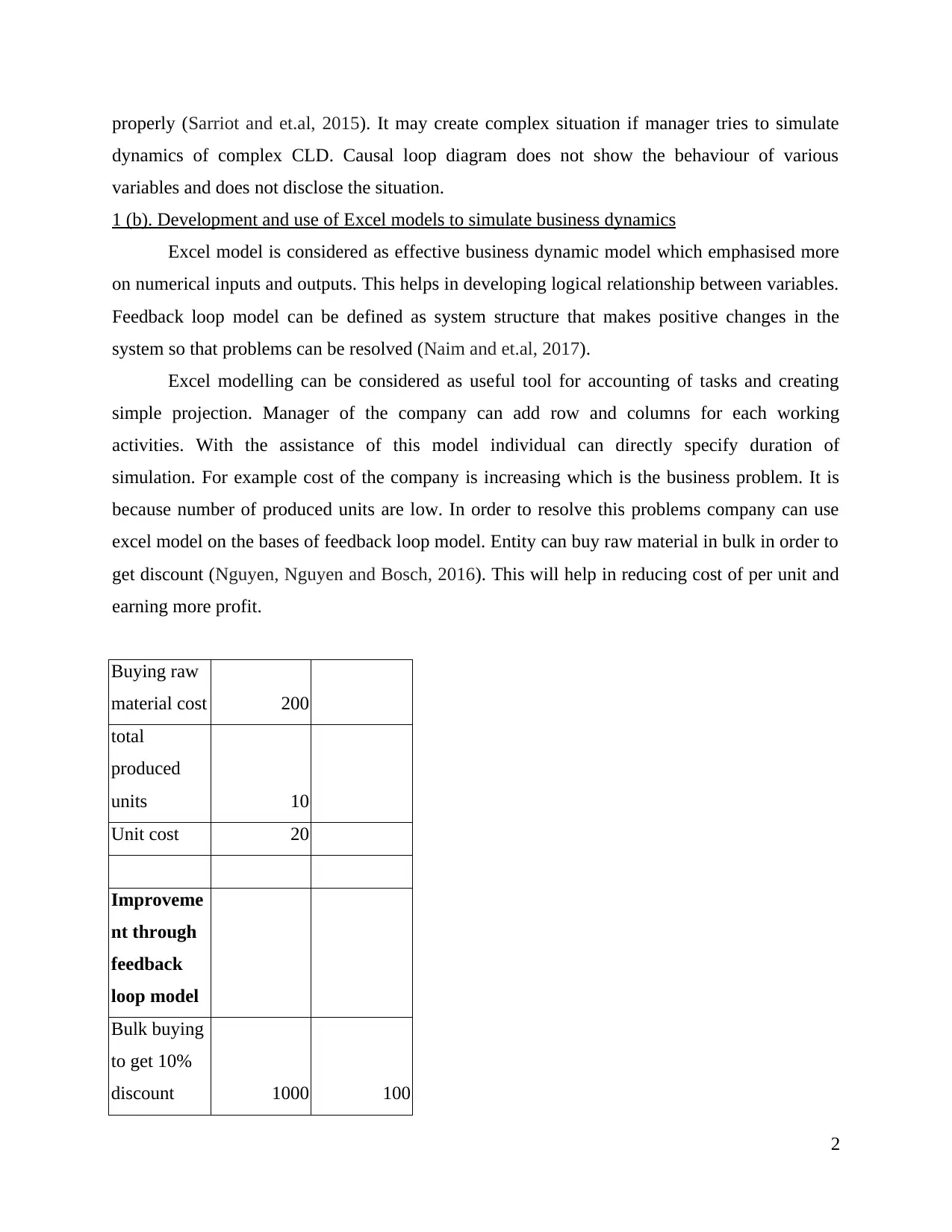
Excel modelling can be considered as useful tool for accounting of tasks and creating
simple projection. Manager of the company can add row and columns for each working
activities. With the assistance of this model individual can directly specify duration of
simulation. For example cost of the company is increasing which is the business problem. It is
because number of produced units are low. In order to resolve this problems company can use
excel model on the bases of feedback loop model. Entity can buy raw material in bulk in order to
get discount (Nguyen, Nguyen and Bosch, 2016). This will help in reducing cost of per unit and
earning more profit.
Buying raw
material cost 200
total
produced
units 10
Unit cost 20
Improveme
nt through
feedback
loop model
Bulk buying
to get 10%
discount 1000 100
2

total
produced
units 10
Unit cost 10
2 (a). Role of supply chain and inventory management
Supply chain management plays significant role in the business system, it supports in
enhancing coordination and improving sequential set of operations in order to reduce
requirement of inventory (Rawlins, Fraser and De Lange, 2015). Supply chain makes
coordination with production, distribution so that efficiency and effectiveness of operations can
be improved. Just in time management technique and inventory control tools help the
organization in making effective control over the business activities. Supply chain plays
significant role because with the assistance of this tool company can decrease purchasing cost
and decrease total supply cost as well. It helps in improving profit leverage and cash flow as well
(Newman and et.al, 2016). On other hand inventory management system assists in keeping
records of inventory orders, maintain stock. Both supply chain and inventory management
techniques helps in making control over unnecessary cost and increasing profit of the entity.
Just in time theory is the beneficial technique which explains that there is no need to
produce extra products until demand gets arisen (Trani and et.al, 2016). It is beneficial in
reducing overhead expenses. Company has to record all stock detail, future demand and
according they have to order new raw material.
2 (b). Use of economic order quantity model and production quantity model
Economic order quantity (EOQ) is the technique that minimize total holding and ordering
cost. There are two main costs are involved in inventory management such as ordering and
holding cost. Total inventory cost ca be analysed by adding both these cost. It is useful model
which helps the organization in minimizing storage and holding cost. It takes support of such
data which can easily be get thus, calculations can be done easily (Jhawar, Garg and Khera,
2017).
Production quantity model is another inventory management model which determines the
quantity of order that needs to be done to minimize inventory cost. It is useful in minimizing
3

total cost which is associated with purchase, storage and delivery. By this way entity can
enhance its profitability (VASS and et.al, 2014).
ECA PART 2
TASK 1
Cause and relationship between linked variables
Causal loop diagram can be explained as system behaviour in which each variable is
connected with others through nodes, this feedback loop creates connection between various
variables. Problems are defined through these nodes, whereas rest nodes explains the cause of
problems. There are mainly two types of loops: reinforce and balancing feedback loop.
Reinforcing feedback loop explains the changes in which one node goes around and loop in same
direction and explains the cause of change. Whereas in balancing loop these goes in opposite
direction. Discrepancies can be defined as gap between actual warehouse inventory and in-store
inventories. If expected record of stock does not match with actual account then it may create
issue of discrepancy. Process 1 is being selected for this section.
By using causal feedback loop model it is identified that In the glass sheet manufacturing
process there is gap between forecasted inventory and desired inventory records (Cárdenas-
Barrón, Chung and Treviño-Garza, 2014). Glass sheet manufacturing process in much more
depended upon the order rate and inventory available in the company. There is strong
relationship between various variables, these parameters impact on others. By analysing cause
and relationship business problems can be identified easily and management can take action to
resolve such type of issues. It helps in analysing relationship between two variables whether they
have direct or inverse relationship. By this way overall performance of the product or factor can
be measured. The cause of the problem is that inventory is not adequate that create issues and
process can not be completed with these lack of stock. This is the main cause of the problem that
is identified through reinforcing feedback loop model. On other hand in order to balance this
problem it is required to have adequate inventory for the glass manufacturing process.
As in the process 1, inventory GS and order rate are highly depended. If order rate gets
increased and company does not have sufficient stock then it may create issues. Due to this it
will not be able to meet with desired demand (Paul and Goswami, 2018). It will affect delivery
timings. On other hand if inventory GS is high and order rate is low then it will create
discrepancy and entity will have to face loss due to imbalance between supply and demand.
4

Production rate and inventory GS is highly related with each others. There is cause and
relationship between production order rate and production rate. There is positive relationship
between both these variables. If order rate is high then company will require to produce more
glass sheet which will enhance production rate to great extent. On other hand if order rate is low
then production rate will get decreased (How to Determine Production Ratio, 2017).
In order to identify relationship between cause and effects this causal loop diagram is
effective. If two nodes are changing in same direction that means here is positive causal link
whereas if they are in opposite direction then it shown negative link between two variables.
There is cause and relationship between delivery timing and production. If order rate is
high then company will have to enhance its production. In the large number of production of
glass sheets there company will require more time to produce it. Due to this delivery timing will
get enhance. If delivery rate is high then production ratio will get affected. In manufacturing
large glass sheet company will require more time thus, ratio will get changed. Furthermore, there
is strong relationship between inventory GS, desired inventory and order rate (Using causal loop
diagram to achieve a better understanding of e-business models, 2009). As order is generated
through cloud, if company has adequate stock as per the required demand then it would be able
to meet with the demand. On other hand if inventory is not sufficient then it may create issue in
the manufacturing because this gap between desired stock and actual stock level can create
consequences. If desired inventory is inadequate and order rate is high then it will affect
production ratio to great extent (Are causal loop diagrams useful?, 2017). Thus, there is direct
relationship between both these variables.
TASK 2
Polarity of causal link
Causal loop diagram explains relationship between cause and effects. As in the selected
process 1 glass manufacturing process it is identified that gap between actual inventory and
expected inventory is here that results negative production rate. Positive sign or S denotes that
two nodes are changing in the same direction. That means strengthening of one variable causes
strength to other variable as well. On other hand negative sign which is denotes through O shows
that strengthening of one variable result in decreasing strengthening of other attributes.
5

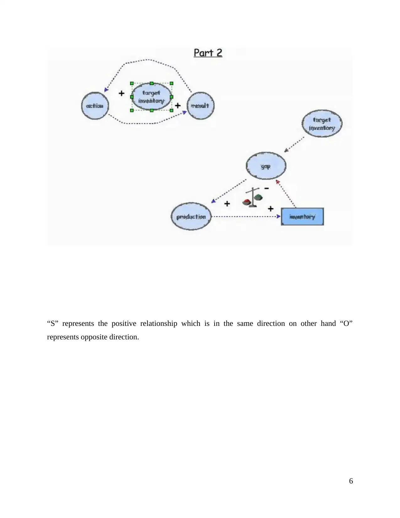
“S” represents the positive relationship which is in the same direction on other hand “O”
represents opposite direction.
6

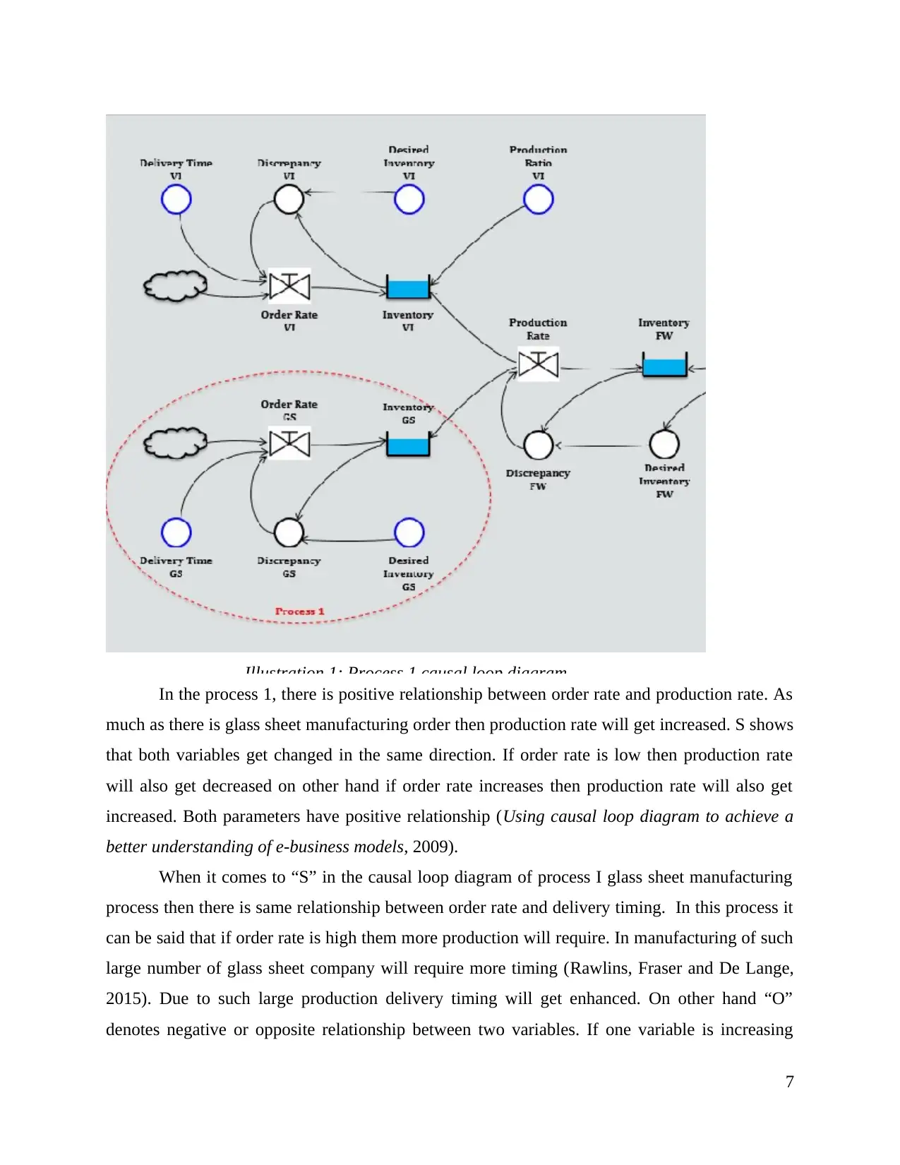
Illustration 1: Process 1 causal loop diagram
In the process 1, there is positive relationship between order rate and production rate. As
much as there is glass sheet manufacturing order then production rate will get increased. S shows
that both variables get changed in the same direction. If order rate is low then production rate
will also get decreased on other hand if order rate increases then production rate will also get
increased. Both parameters have positive relationship (Using causal loop diagram to achieve a
better understanding of e-business models, 2009).
When it comes to “S” in the causal loop diagram of process I glass sheet manufacturing
process then there is same relationship between order rate and delivery timing. In this process it
can be said that if order rate is high them more production will require. In manufacturing of such
large number of glass sheet company will require more timing (Rawlins, Fraser and De Lange,
2015). Due to such large production delivery timing will get enhanced. On other hand “O”
denotes negative or opposite relationship between two variables. If one variable is increasing
7

then other will get decreased. There is O polarity between inventory and production rate. If
production rate is increasing which means stock available to the warehouse is decreasing. If
demand is high then company will require more inventory because existing stock will not be able
to meet with the demand rate (Naim and et.al, 2017). Thus, there is opposite polarity between
production rate and inventory. If production is decreasing them available inventory will remain
same it will not get decreased. If forecasted demand is high as compare to actual order rate then
inventory GS will be low. It shows opposite polarity between both variables. Company always
keeps stock in warehouse as per the required demand. But if there is difference between
forecasted order rate and actual order rate then it will create discrepancy in inventory. Because
available stock will not be adequate to meet this demand (Sarriot and et.al, 2015).
TASK 3
Calculations for each variable
There are various variables that impact on the total results. As simulation model analyse
current performance by looking at the expected performance of the process. As in the process 1
of glass manufacturing process there are two main variables that are linked with each others.
They both impact on each others as both they have strong relationship with each others. It has
been identified that gap between actual and expected inventory impact on overall production
capacity of the process. If available inventory is not enough then it would not be able to met with
the demand. That main create consequence. Thus, it is essential to make balance between two
variables. Example of current situation are as discussed below:
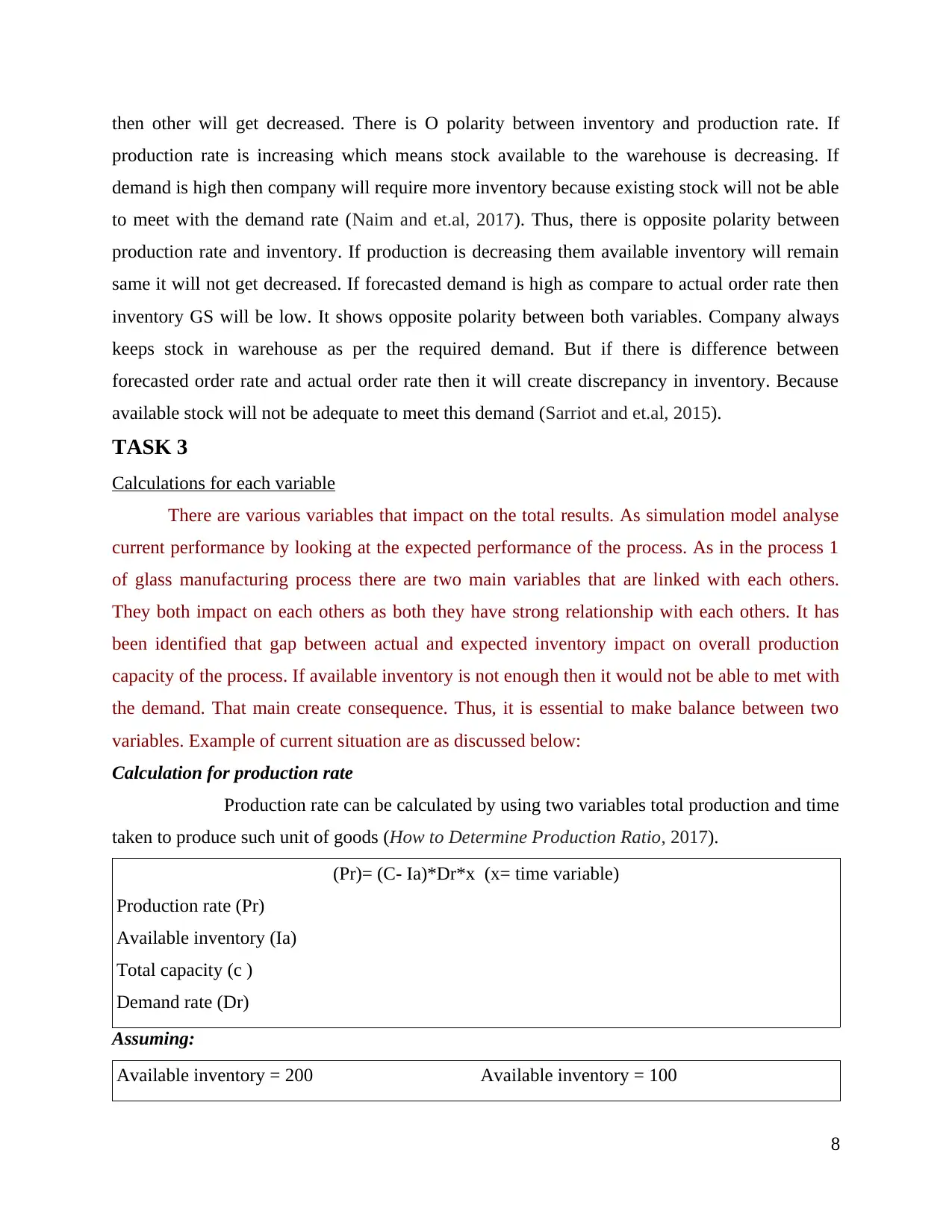
Calculation for production rate
Production rate can be calculated by using two variables total production and time
taken to produce such unit of goods (How to Determine Production Ratio, 2017).
(Pr)= (C- Ia)*Dr*x (x= time variable)
Production rate (Pr)
Available inventory (Ia)
Total capacity (c )
Demand rate (Dr)
Assuming:
Available inventory = 200 Available inventory = 100
8

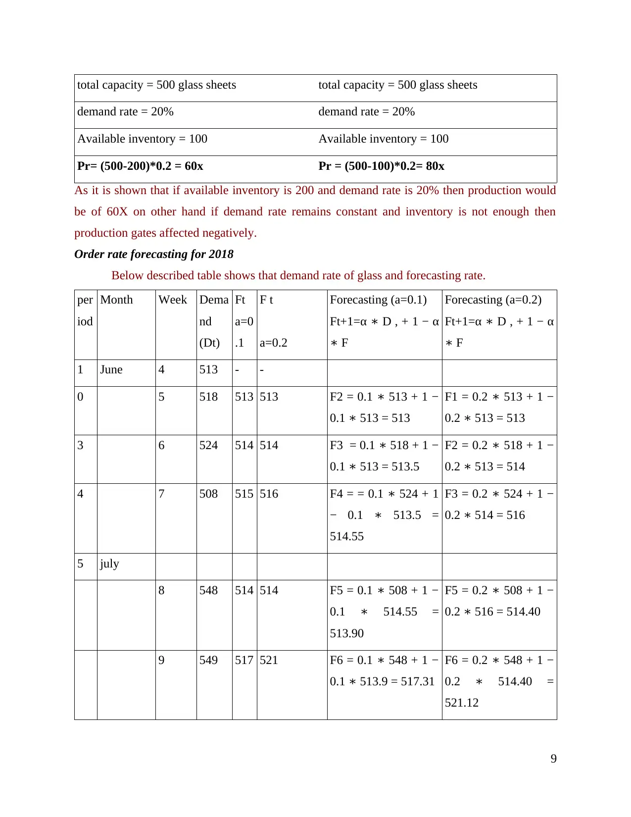
total capacity = 500 glass sheets total capacity = 500 glass sheets
demand rate = 20% demand rate = 20%
Available inventory = 100 Available inventory = 100
Pr= (500-200)*0.2 = 60x Pr = (500-100)*0.2= 80x
As it is shown that if available inventory is 200 and demand rate is 20% then production would
be of 60X on other hand if demand rate remains constant and inventory is not enough then
production gates affected negatively.
Order rate forecasting for 2018
Below described table shows that demand rate of glass and forecasting rate.
per
iod
Month Week Dema
nd
(Dt)
Ft
a=0
.1
F t
a=0.2
Forecasting (a=0.1)
Ft+1=α D , + 1 − α∗
F∗
Forecasting (a=0.2)
Ft+1=α D , + 1 − α∗
F∗
1 June 4 513 - -
0 5 518 513 513 F2 = 0.1 513 + 1 −∗
0.1 513 = 513∗
F1 = 0.2 513 + 1 −∗
0.2 513 = 513∗
3 6 524 514 514 F3 = 0.1 518 + 1 −∗
0.1 513 = 513.5∗
F2 = 0.2 518 + 1 −∗
0.2 513 = 514∗
4 7 508 515 516 F4 = = 0.1 524 + 1∗
− 0.1 513.5 =∗
514.55
F3 = 0.2 524 + 1 −∗
0.2 514 = 516∗
5 july
8 548 514 514 F5 = 0.1 508 + 1 −∗
0.1 514.55 =∗
513.90
F5 = 0.2 508 + 1 −∗
0.2 516 = 514.40∗
9 549 517 521 F6 = 0.1 548 + 1 −∗
0.1 513.9 = 517.31∗
F6 = 0.2 548 + 1 −∗
0.2 514.40 =∗
521.12
9

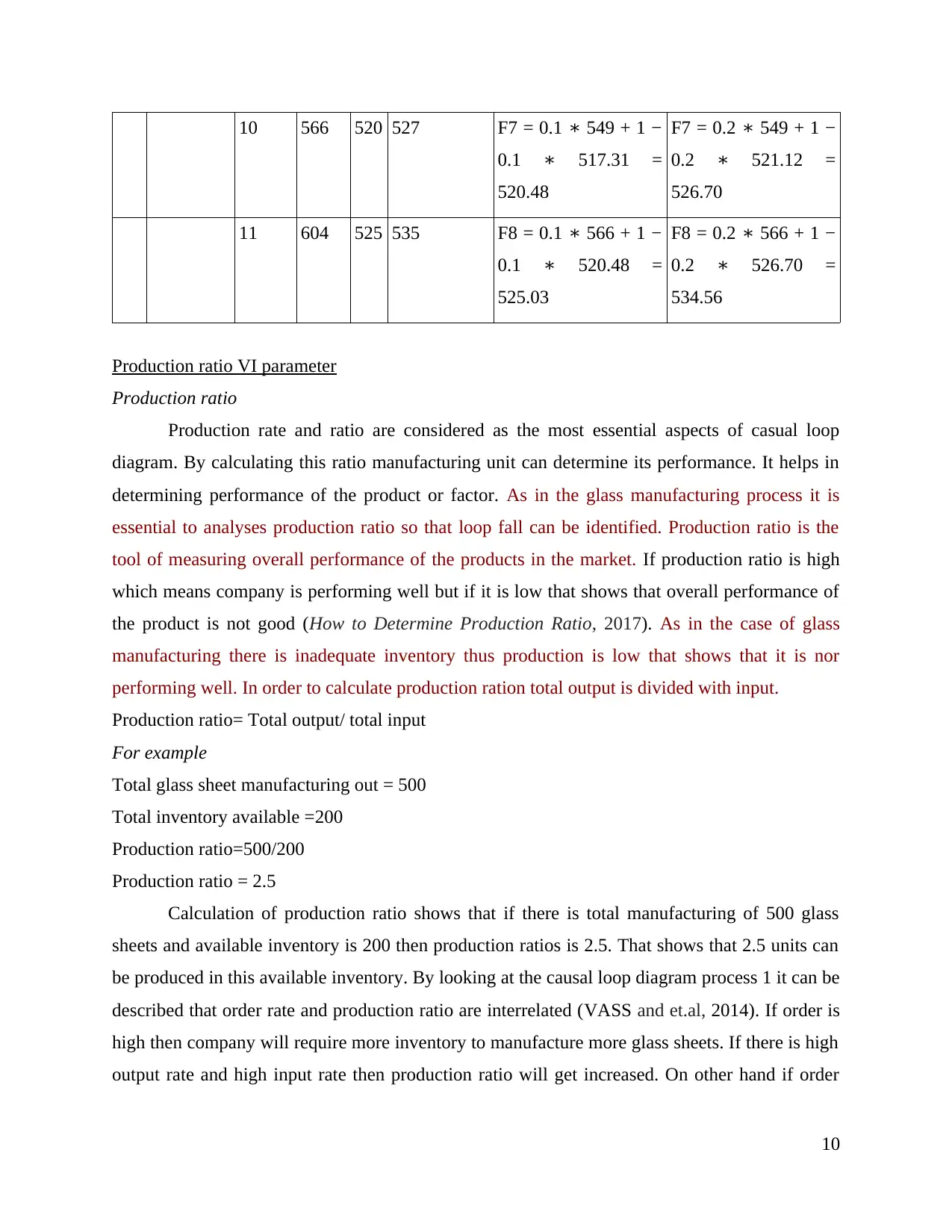
10 566 520 527 F7 = 0.1 549 + 1 −∗
0.1 517.31 =∗
520.48
F7 = 0.2 549 + 1 −∗
0.2 521.12 =∗
526.70
11 604 525 535 F8 = 0.1 566 + 1 −∗
0.1 520.48 =∗
525.03
F8 = 0.2 566 + 1 −∗
0.2 526.70 =∗
534.56
Production ratio VI parameter
Production ratio
Production rate and ratio are considered as the most essential aspects of casual loop
diagram. By calculating this ratio manufacturing unit can determine its performance. It helps in
determining performance of the product or factor. As in the glass manufacturing process it is
essential to analyses production ratio so that loop fall can be identified. Production ratio is the
tool of measuring overall performance of the products in the market. If production ratio is high
which means company is performing well but if it is low that shows that overall performance of
the product is not good (How to Determine Production Ratio, 2017). As in the case of glass
manufacturing there is inadequate inventory thus production is low that shows that it is nor
performing well. In order to calculate production ration total output is divided with input.
Production ratio= Total output/ total input
For example
Total glass sheet manufacturing out = 500
Total inventory available =200
Production ratio=500/200
Production ratio = 2.5
Calculation of production ratio shows that if there is total manufacturing of 500 glass
sheets and available inventory is 200 then production ratios is 2.5. That shows that 2.5 units can
be produced in this available inventory. By looking at the causal loop diagram process 1 it can be
described that order rate and production ratio are interrelated (VASS and et.al, 2014). If order is
high then company will require more inventory to manufacture more glass sheets. If there is high
output rate and high input rate then production ratio will get increased. On other hand if order
10

rate is high but there is discrepancy in available inventory or there is inadequate stock available
then production ratio will get decreased (Paul and Goswami, 2018).
Process 1 casual loop diagram shows that there is relationship between order rate,
inventory and production ratio. If order rate is high and there is inadequate inventory available
then it may create discrepancy. In such condition manufacture will have to include more input to
meet with the desired inventory quantity. For example if desired inventory quantity is 250 and
total manufacturing of glass sheet would be 500 then production ratios would be 500/250= 2.
Thus, discrepancy between desired inventory and actual stock level impact on the production
ratio to great extent (Cárdenas-Barrón, Chung and Treviño-Garza, 2014).
CONCLUSION
From the above study it can be concluded that causal loop diagram shows the connection
between various variables through nodes. It helps in analysing the business problem and finding
cause and relationship between two parameters. There are direct and inverse relationship
between several variables. If there is positive or direct relationship that means both variables will
get influenced in the same direction, if one factor is increasing them other will also get increased.
On other hand inverse relationship shows that if one variable is increasing then other will get
decreased. This interconnection supports in calculating production rate and production ratio.
That helps in identifying the root cause of problems and making balance between demand and
supply.
11

REFERENCES
Books and Journals
Cárdenas-Barrón, L. E., Chung, K. J. and Treviño-Garza, G., 2014. Celebrating a century of the
economic order quantity model in honor of Ford Whitman Harris.
Cavana, R. Y. and et.al., 2014. Causal mapping of the New Zealand natural resources sector
system: A preliminary analysis. InProceedings of the 2014 International System Dynamics
Conference, System Dynamics Society, Chestnut Hill.
Jhawar, A., Garg, S. K. and Khera, S. N., 2017. Improving logistics performance through
investments and policy intervention: a causal loop model. International Journal of
Productivity and Quality Management. 20(3). pp.363-391.
Naim, M. M. and et.al., 2017. Identifying the causes of the bullwhip effect by exploiting control
block diagram manipulation with analogical reasoning.European Journal of Operational
Research.
Newman, R. and et.al., 2016. Model and experimental development for business data
science. International Journal of Information Management. 36(4). pp.607-617.
Nguyen, T. V., Nguyen, N. C. and Bosch, O. J., 2016, January. Developing causal loop diagrams
for coffee supply chain: supporting to enhance the competitive advantages of a vietnamese
coffee. In Proceedings of the 59th Annual Meeting of the ISSS-2015 Berlin, Germany (Vol.
1, No. 1).
Paul, A. and Goswami, A., 2018. An Economic Order Quantity Model for Deteriorating Items
with Ramp Type Demand, Time Dependent Holding Cost and Price Discount Offered on
Backorders. World Academy of Science, Engineering and Technology, International
Journal of Mathematical and Computational Sciences. 5(1).
Rawlins, J. M., Fraser, G. and De Lange, W. J., 2015. Exploring the suitability of causal loop
diagrams to assess the Value chains of aquatic ecosystem services: A case study of the
Baviaanskloof, South Africa.
Sarriot, E. and et.al., 2015. A causal loop analysis of the sustainability of integrated community
case management in Rwanda. Social Science & Medicine. 131. pp.147-155.
12

Trani, J. F. and et.al., 2016. Community based system dynamic as an approach for understanding
and acting on messy problems: a case study for global mental health intervention in
Afghanistan. Conflict and health. 10(1). pp.25.
VASS, H. E. and et.al.,2014. Studiu de caz privind utilizarea în managementul serviciilor de
urgenţă a metodologiei dinamicii sistemelor. Review of Management & Economic
Engineering. 13(1).
Online
Are causal loop diagrams useful?, 2017. [Online]. Available through
<http://metasd.com/2010/04/are-causal-loop-diagrams-useful/>
How to Determine Production Ratio, 2017. [Online]. Available through
<https://bizfluent.com/how-8614580-determine-production-ratio.html>
Using causal loop diagram to achieve a better understanding of e-business models, 2009.
[Online]. Available through
<https://pdfs.semanticscholar.org/62bc/509fb1da7bd300d669dd446846613fd8f070.pdf>
13