Business Economics Assignment: PoolVac Inc. Cost and Demand Analysis

This assignment analyzes the cost structure and demand for PoolVac Inc.'s "Sting Ray" pool cleaner. It begins by estimating the average variable cost (AVC) function using a quadratic specification and calculating total variable cost and marginal cost. The assignment then uses time series modeling to forecast demand, incorporating dummy variables for quarterly variations. Furthermore, a demand function is estimated using multiple regression, considering the product's price, average household income, and the price of a competitor's product. The analysis includes interpreting the statistical significance of the parameters and determining the impact of each variable on quantity demanded. Finally, the assignment derives a price function based on the estimated demand function. The document includes references to relevant economic literature.

Running head: BUSINESS ECONOMICS
Business Economics
Student’s Name
Institution
Date

BUSINESS ECONOMICS 2
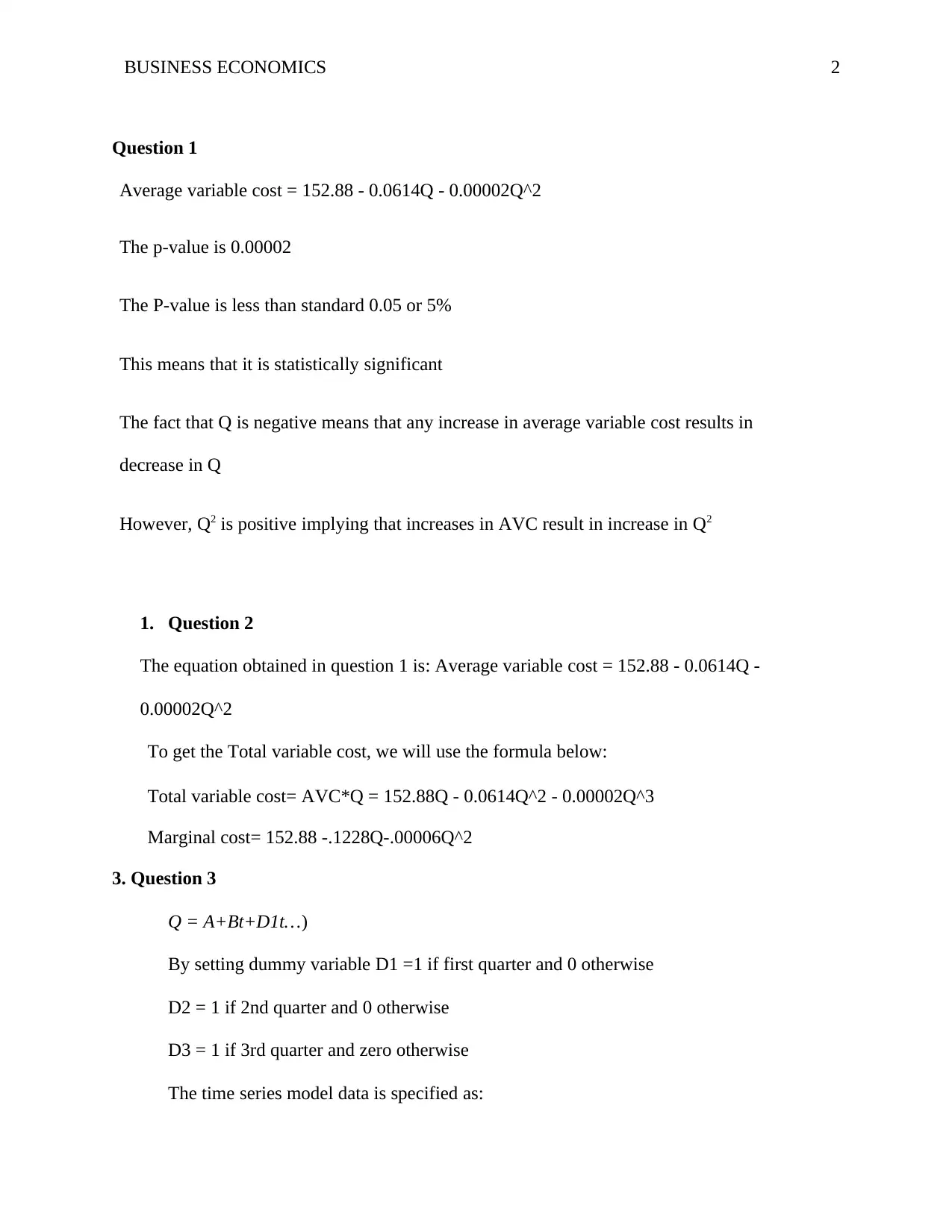
Question 1
Average variable cost = 152.88 - 0.0614Q - 0.00002Q^2
The p-value is 0.00002
The P-value is less than standard 0.05 or 5%
This means that it is statistically significant
The fact that Q is negative means that any increase in average variable cost results in
decrease in Q
However, Q2 is positive implying that increases in AVC result in increase in Q2
1. Question 2
The equation obtained in question 1 is: Average variable cost = 152.88 - 0.0614Q -
0.00002Q^2
To get the Total variable cost, we will use the formula below:
Total variable cost= AVC*Q = 152.88Q - 0.0614Q^2 - 0.00002Q^3
Marginal cost= 152.88 -.1228Q-.00006Q^2
3. Question 3
Q = A+Bt+D1t…)
By setting dummy variable D1 =1 if first quarter and 0 otherwise
D2 = 1 if 2nd quarter and 0 otherwise
D3 = 1 if 3rd quarter and zero otherwise
The time series model data is specified as:

BUSINESS ECONOMICS 3
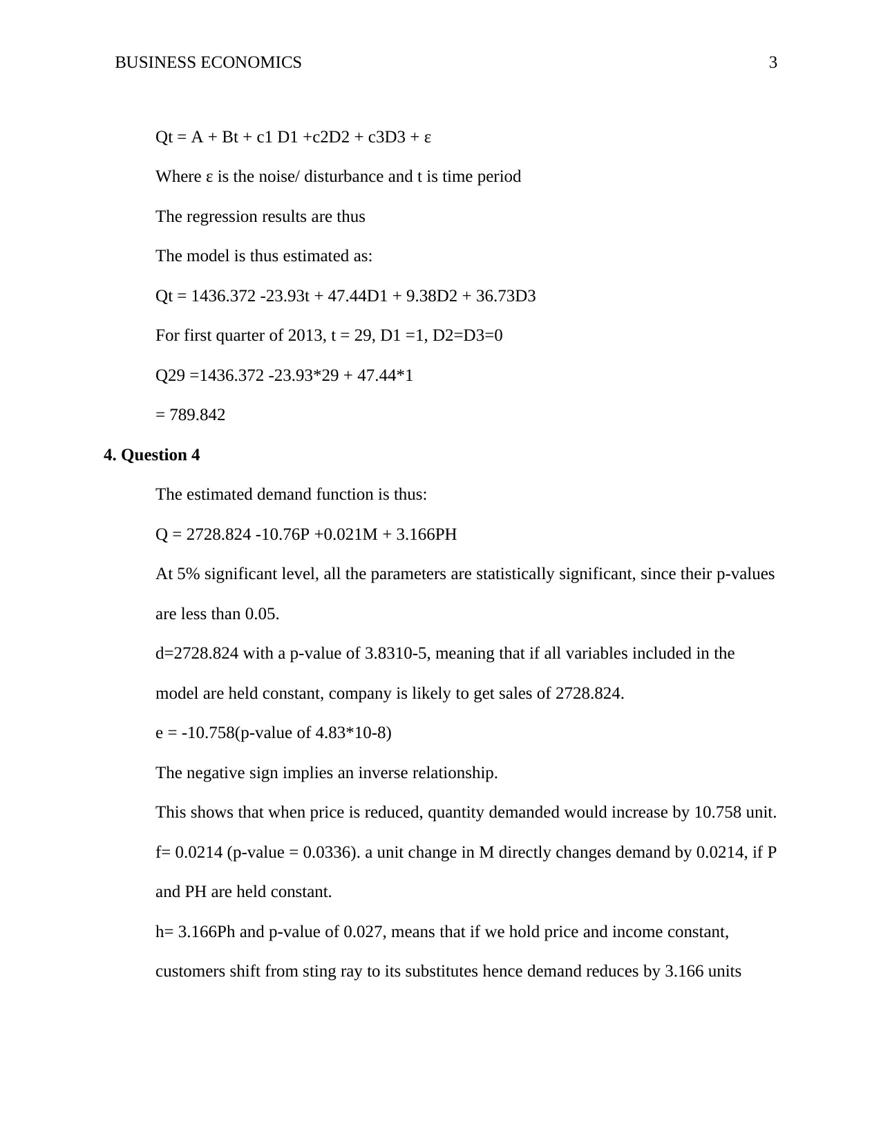
Qt = A + Bt + c1 D1 +c2D2 + c3D3 + ε
Where ε is the noise/ disturbance and t is time period
The regression results are thus
The model is thus estimated as:
Qt = 1436.372 -23.93t + 47.44D1 + 9.38D2 + 36.73D3
For first quarter of 2013, t = 29, D1 =1, D2=D3=0
Q29 =1436.372 -23.93*29 + 47.44*1
= 789.842
4. Question 4
The estimated demand function is thus:
Q = 2728.824 -10.76P +0.021M + 3.166PH
At 5% significant level, all the parameters are statistically significant, since their p-values
are less than 0.05.
d=2728.824 with a p-value of 3.8310-5, meaning that if all variables included in the
model are held constant, company is likely to get sales of 2728.824.
e = -10.758(p-value of 4.83*10-8)
The negative sign implies an inverse relationship.
This shows that when price is reduced, quantity demanded would increase by 10.758 unit.
f= 0.0214 (p-value = 0.0336). a unit change in M directly changes demand by 0.0214, if P
and PH are held constant.
h= 3.166Ph and p-value of 0.027, means that if we hold price and income constant,
customers shift from sting ray to its substitutes hence demand reduces by 3.166 units

BUSINESS ECONOMICS 4
Generally, the three slope parameters, which include parameter for price, income
and cross price are crucial because they determine whether the quantity demanded will go
up or down. If the parameter has negative sign, it will mean that quantity demanded
would be high.
5. Question 5
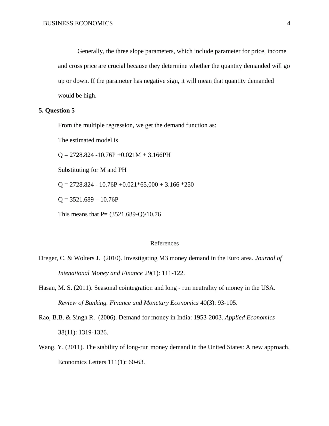
From the multiple regression, we get the demand function as:
The estimated model is
Q = 2728.824 -10.76P +0.021M + 3.166PH
Substituting for M and PH
Q = 2728.824 - 10.76P +0.021*65,000 + 3.166 *250
Q = 3521.689 – 10.76P
This means that P= (3521.689-Q)/10.76
References
Dreger, C. & Wolters J. (2010). Investigating M3 money demand in the Euro area. Journal of
Intenational Money and Finance 29(1): 111-122.
Hasan, M. S. (2011). Seasonal cointegration and long - run neutrality of money in the USA.
Review of Banking. Finance and Monetary Economics 40(3): 93-105.
Rao, B.B. & Singh R. (2006). Demand for money in India: 1953-2003. Applied Economics
38(11): 1319-1326.
Wang, Y. (2011). The stability of long-run money demand in the United States: A new approach.
Economics Letters 111(1): 60-63.