Comprehensive Business Economics Assignment Solution
VerifiedAdded on 2021/06/16
|15
|2610
|24
Homework Assignment
AI Summary
This document presents a comprehensive solution to a business economics assignment. It begins by defining and analyzing allocative efficiency in both perfectly competitive and monopolistically competitive markets, illustrating the concepts with relevant figures. The assignment then delves into market-based instruments for environmental policy, specifically transferable pollution permits and taxes, explaining their mechanisms and effects. Further, it examines supply curves in increasing and constant cost industries, providing graphical representations. Finally, the solution explores elasticity concepts, including income and cross-price elasticity, and classifies goods as normal or inferior based on elasticity measures, offering practical examples and interpretations. The document is well-structured, includes diagrams, and provides a detailed analysis of each concept.

Running Head: BUSINESS ECONOMICS
Business Economics
Name of the Student
Name of the University
Course ID
Business Economics
Name of the Student
Name of the University
Course ID
Paraphrase This Document
Need a fresh take? Get an instant paraphrase of this document with our AI Paraphraser

1BUSINESS ECONOMICS
Table of Contents
Answer 1..........................................................................................................................................2
Answer a......................................................................................................................................2
Answer b......................................................................................................................................3
Answer 5..........................................................................................................................................4
Answer 7..........................................................................................................................................7
Answer 8..........................................................................................................................................9
Answer a......................................................................................................................................9
Answer b....................................................................................................................................10
Answer c....................................................................................................................................10
Answer d....................................................................................................................................11
Answer 9........................................................................................................................................12
Answer a....................................................................................................................................12
Answer b....................................................................................................................................12
Answer c....................................................................................................................................12
Answer d....................................................................................................................................12
Answer e....................................................................................................................................12
Answer f.....................................................................................................................................12
Answer g....................................................................................................................................13
Answer h....................................................................................................................................13
Answer i.....................................................................................................................................13
Reference list.................................................................................................................................14

2BUSINESS ECONOMICS
Answer 1
Answer a
Allocative Efficiency
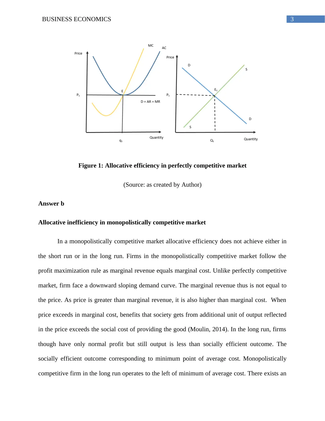
Allocative efficiency refers to the choice of production points on the production
possibility curve such that the points are socially preferred. Perfectly competitive firm is taken as
a benchmark for allocative efficiency. In perfectly competitive market, the price that prevails in
the market always equals to the marginal cost of production. For a particular good price is used
as a signal for social benefit. The marginal cost on the other hand not only represents cost of
seller but is also a representative measure social cost of the good (Fine, 2016). By following the
profit maximizing rule of price equals marginal cost competitive firms ensure allocative
efficiency.
Perfectly competitive market and allocative efficiency
In a perfectly competitive industry, all the firm in the long run can enjoy only a normal
profit. Suppose a competitive firm in the long run is enjoying a supernormal profit. It then
encourages other firms to enter the industry. Entry of new firms continue until only normal profit
is left in the industry. During economic loss, firms leave the industry (Baumol & Blinder, 2015).
The long run equilibrium holds where price equals minimum average cost which also equal
marginal cost.
Answer 1
Answer a
Allocative Efficiency
Allocative efficiency refers to the choice of production points on the production
possibility curve such that the points are socially preferred. Perfectly competitive firm is taken as
a benchmark for allocative efficiency. In perfectly competitive market, the price that prevails in
the market always equals to the marginal cost of production. For a particular good price is used
as a signal for social benefit. The marginal cost on the other hand not only represents cost of
seller but is also a representative measure social cost of the good (Fine, 2016). By following the
profit maximizing rule of price equals marginal cost competitive firms ensure allocative
efficiency.
Perfectly competitive market and allocative efficiency
In a perfectly competitive industry, all the firm in the long run can enjoy only a normal
profit. Suppose a competitive firm in the long run is enjoying a supernormal profit. It then
encourages other firms to enter the industry. Entry of new firms continue until only normal profit
is left in the industry. During economic loss, firms leave the industry (Baumol & Blinder, 2015).
The long run equilibrium holds where price equals minimum average cost which also equal
marginal cost.
⊘ This is a preview!⊘
Do you want full access?
Subscribe today to unlock all pages.
Trusted by 1+ million students worldwide
3BUSINESS ECONOMICS
Figure 1: Allocative efficiency in perfectly competitive market
(Source: as created by Author)
Answer b
Allocative inefficiency in monopolistically competitive market
In a monopolistically competitive market allocative efficiency does not achieve either in
the short run or in the long run. Firms in the monopolistically competitive market follow the
profit maximization rule as marginal revenue equals marginal cost. Unlike perfectly competitive
market, firm face a downward sloping demand curve. The marginal revenue thus is not equal to
the price. As price is greater than marginal revenue, it is also higher than marginal cost. When
price exceeds in marginal cost, benefits that society gets from additional unit of output reflected
in the price exceeds the social cost of providing the good (Moulin, 2014). In the long run, firms
though have only normal profit but still output is less than socially efficient outcome. The
socially efficient outcome corresponding to minimum point of average cost. Monopolistically
competitive firm in the long run operates to the left of minimum of average cost. There exists an
Paraphrase This Document
Need a fresh take? Get an instant paraphrase of this document with our AI Paraphraser

4BUSINESS ECONOMICS
excess capacity in the industry. In the monopolistically competitive market, firms using its
market power produce a lower quantity and charges a higher price. This explains existence of
allocative inefficiency in monopolistically competitive market.
Figure 2: Allocative inefficiency in monopolistically competitive market
(Source: as created by Author)
Answer 5
In designing environmental policy, the market based instruments are defined as policy
tools that works through market mechanism and use price or other economic variables in order
to provide incentive to the polluters for eliminating or reducing negative externality harming the
environment. It is a self-correction mechanism that addresses the problem of market failure
resulted from externality.
Two commonly used market mechanism used for controlling pollution as an externality is tax
and transferrable pollution permit.

5BUSINESS ECONOMICS
Transferable permits
The mechanism of transferable pollution permit sets a certain level of pollution. This
provides firms a legal right to pollute the set amount of pollution. It is possible for some firms to
reduce pollution at a lower cost than others. As the concerned firm can reduce pollution at a
lower cost it trades the permit to other firms. Others who are unable to reduce the level of
pollution demand permits from other firms or government (Friedman, 2017). This creates a
market of pollution permit where permits are traded at certain prices. Objective of the pollution
permit is to offer market incentive to firms to internalize the external cost of pollution.
Figure 3: Market for pollution permit
(Source: ac created by Author)
In the market for pollution permit, the supply of permits fixed at Q1. The demand for permit
depends on the firms’ ability to reduce pollution. If the demand for pollution increases then
⊘ This is a preview!⊘
Do you want full access?
Subscribe today to unlock all pages.
Trusted by 1+ million students worldwide

6BUSINESS ECONOMICS
demand curve shifts from DD to D1D1 leading to an increase in cost of permits from P1 to P2.
Firms therefore has own incentive to reduce pollution rather than paying a high price to obtain
tradable permits.
Tax
Under the market based approach of tax, the maximum cost for implementing pollution
control measures are determined. The polluters here have an incentive to lower pollution at a
relatively low cost rather than paying a tax. Unlike pollution permits, no upper limit is set for
pollution. The level of pollution rather depends on the implemented tax rate. The imposed tax is
generally equivalent to the external cost determined from the difference between marginal social
cost and marginal private cost (Cowen & Tabarrok, 2015).
Figure 4: Effect of a tax on pollution
(Source: as created by Author)
S1 curve shows the marginal private cost of the polluting firm. The D1 curve shows marginal
benefit as usual. The free market equilibrium is at E indicating market price and quantity as P1
Paraphrase This Document
Need a fresh take? Get an instant paraphrase of this document with our AI Paraphraser
7BUSINESS ECONOMICS
and Q1 respectively. In the presence of negative externality of pollution social marginal cost
exceeds the private marginal cost. Now, imposition of a tax of ‘t’ equivalent to external cost
shifts the supply curve upwards to S2. This reduces pollution to Q2 and raise price to P2. This is
how tax works in combating pollution.
Answer 7
Supply Curve in an increasing cost industry
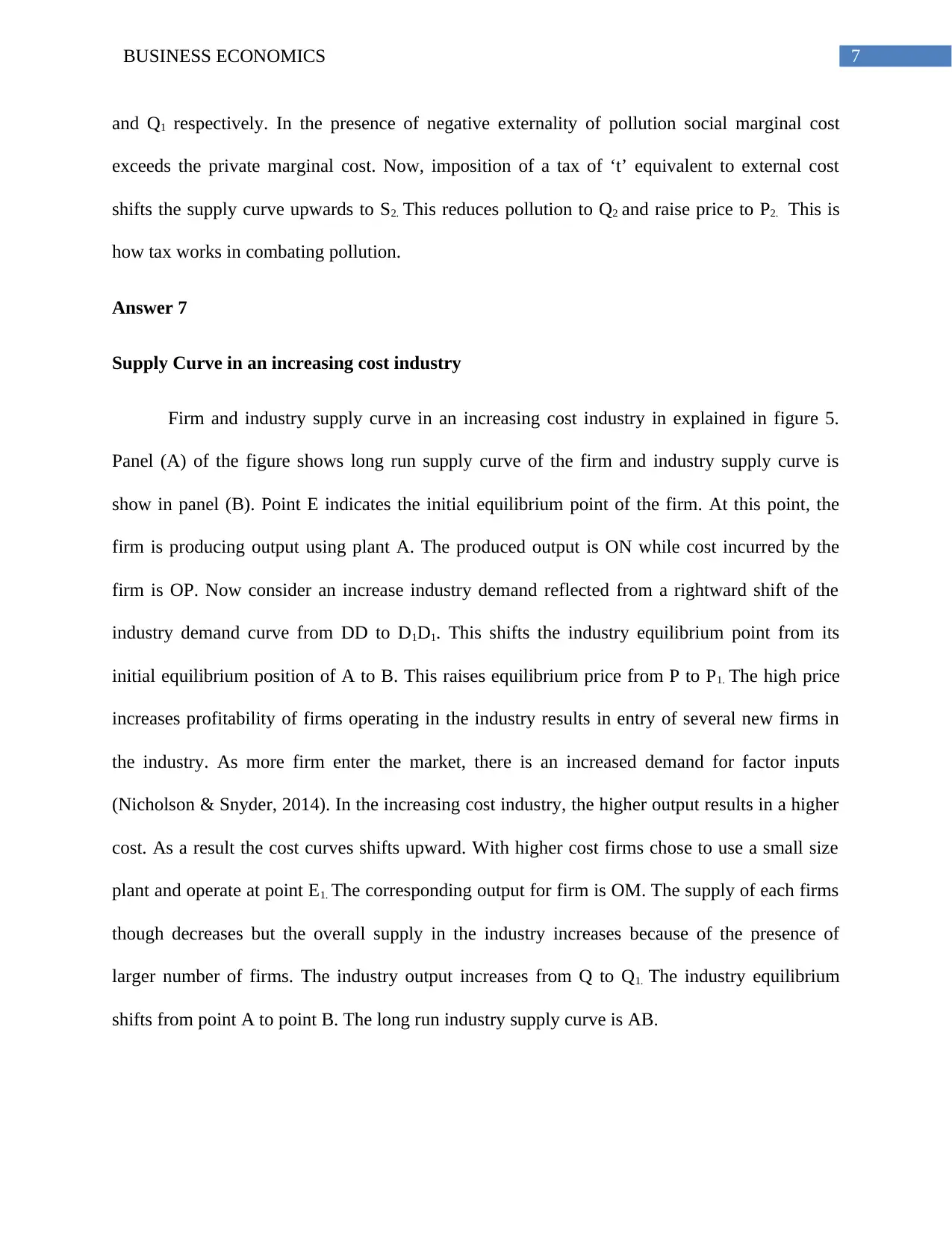
Firm and industry supply curve in an increasing cost industry in explained in figure 5.
Panel (A) of the figure shows long run supply curve of the firm and industry supply curve is
show in panel (B). Point E indicates the initial equilibrium point of the firm. At this point, the
firm is producing output using plant A. The produced output is ON while cost incurred by the
firm is OP. Now consider an increase industry demand reflected from a rightward shift of the
industry demand curve from DD to D1D1. This shifts the industry equilibrium point from its
initial equilibrium position of A to B. This raises equilibrium price from P to P1. The high price
increases profitability of firms operating in the industry results in entry of several new firms in
the industry. As more firm enter the market, there is an increased demand for factor inputs
(Nicholson & Snyder, 2014). In the increasing cost industry, the higher output results in a higher
cost. As a result the cost curves shifts upward. With higher cost firms chose to use a small size
plant and operate at point E1. The corresponding output for firm is OM. The supply of each firms
though decreases but the overall supply in the industry increases because of the presence of
larger number of firms. The industry output increases from Q to Q1. The industry equilibrium
shifts from point A to point B. The long run industry supply curve is AB.
and Q1 respectively. In the presence of negative externality of pollution social marginal cost
exceeds the private marginal cost. Now, imposition of a tax of ‘t’ equivalent to external cost
shifts the supply curve upwards to S2. This reduces pollution to Q2 and raise price to P2. This is
how tax works in combating pollution.
Answer 7
Supply Curve in an increasing cost industry
Firm and industry supply curve in an increasing cost industry in explained in figure 5.
Panel (A) of the figure shows long run supply curve of the firm and industry supply curve is
show in panel (B). Point E indicates the initial equilibrium point of the firm. At this point, the
firm is producing output using plant A. The produced output is ON while cost incurred by the
firm is OP. Now consider an increase industry demand reflected from a rightward shift of the
industry demand curve from DD to D1D1. This shifts the industry equilibrium point from its
initial equilibrium position of A to B. This raises equilibrium price from P to P1. The high price
increases profitability of firms operating in the industry results in entry of several new firms in
the industry. As more firm enter the market, there is an increased demand for factor inputs
(Nicholson & Snyder, 2014). In the increasing cost industry, the higher output results in a higher
cost. As a result the cost curves shifts upward. With higher cost firms chose to use a small size
plant and operate at point E1. The corresponding output for firm is OM. The supply of each firms
though decreases but the overall supply in the industry increases because of the presence of
larger number of firms. The industry output increases from Q to Q1. The industry equilibrium
shifts from point A to point B. The long run industry supply curve is AB.
8BUSINESS ECONOMICS
Figure 5: Supply curve and increasing cost industry
(Source: as created by Author)
Supply Curve in a constant cost industry
Figure 6 explains the long run supply curve for the firm and industry with a constant cost
of operation. As before, panel (A) shows revenue, cost and supply of the firm while panel (B)
shows the same for the industry. The firm is in equilibrium at point E producing OM output. The
corresponding equilibrium for the industry is at A. The increase in industry demand again raise
price and attracts new firms to enter the market. The entry of new firms does not change the cost
condition. The cost curves do not shift upward and the firms continue to operate with same LAC.
The entry of new firms just shift the industry supply curve to the right (Mochrie, 2015). The new
⊘ This is a preview!⊘
Do you want full access?
Subscribe today to unlock all pages.
Trusted by 1+ million students worldwide

9BUSINESS ECONOMICS
industry equilibrium point is at B. At the new equilibrium, output increases both for firm and the
industry. The long run supply curve in a constant cost industry is thus a horizontal straight line.
Figure 6: Long run Supply curve and constant cost industry
(Source: as created by Author)
Answer 8
Answer a
Income elasticity measures the percentage change in quantity demanded in response to a
corresponding percentage change in income (Fine, 2016). From the measure of income elasticity,
the expected change in demand can be estimated for an expected change in income. The income
elasticity for pre-recorded music compact disc is +7. This means 1 percent change in income will
lead to a 7% increases in demand for pre-recorded music compact disc. Therefore, the economic
Paraphrase This Document
Need a fresh take? Get an instant paraphrase of this document with our AI Paraphraser

10BUSINESS ECONOMICS
expansion that increases consumer income by 10% will result in a (10*7) = 70% increase in
demand pre-recorded music disk. For cabinet maker the income elasticity is 0.7. 10% increase in
income resulted from economic expansion thus can increase the demand by (0.7 * 10) = 7%.
Increases consumers income by 10% thus results in a greater proportionate increase in demand
for pre-recorded music disk as compared to cabinet makers. The sales of pre-recorded music disk
will increase more than that for cabinet makers after increase in income.
Answer b
A simple way to understand whether pre-recorded music disk and MP3 player are in
competition or not is to compute the cross price elasticity of demand. The cross price elasticity
captures percentage change in demand for a corresponding proportionate change in price of some
related good. A positive value of cross price elasticity implies that an increases in price of any
one of them though have an adverse effect on its own demand but have a favorable impact on
demand of the other. In this case the two products are identified as substitute to each other and
hence, intense competition exists between them (Ashwin, Taylor & Mankiw, 2016). A positive
value of cross price elasticity on the other hand implies that the products are complementary to
each other and hence, there is no competition.
Answer c
A good can be classified as normal or inferior depending on the relation between demand
and income. A positive relation between demand and income implies the good is a normal good.
On the other hand, if demand falls along with an increase in income then the good is inferior
(Friedman, 2017).
11BUSINESS ECONOMICS
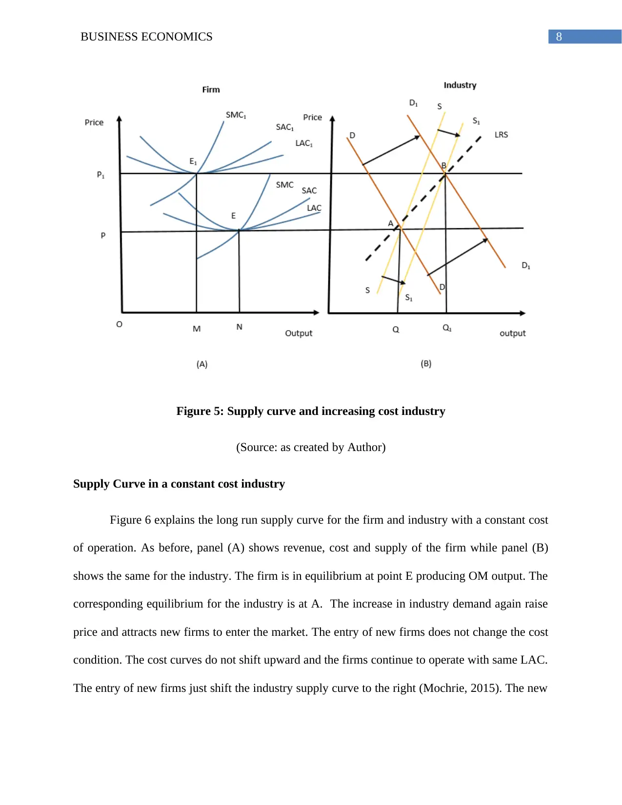
YED = +0.6
This implies one percent increase in income leads to a 0.6% increase in demand. The
proportionate increase in demand is less than the proportionate increases income. The good thus
relatively income inelastic. As demand increases with increase in income, this is a normal good.
The elasticity is less than one implying the good is a necessary one.
YED = -2.6.
The income elasticity measure indicates that 1 percent increase in demand causes a 2.6%
decrease in demand. As demand decreases with an increase in income the good is an inferior
good. The measured elasticity in greater than 1 implying proportionate change in demand is
much greater than that of income. The demand thus is relatively income elastic.
Answer d
XED = +0.64.
The estimated elasticity indicates 1% increase in price of the related good lead to a 0.64%
increase in demand for the concerned good. The positive cross price elasticity implies that
demand for the good increases when price of the related good increases. This is the case for
substitute goods. The two goods in the question is thus substitute to each other. When price of a
good increases, demand for the good goes down while demand for the substitute goods increases.
This explains the positive cross price elasticity for substitute goods.
XED = -2.6
The elasticity measure implies 1% increase in price of the related good lead to a 2.6% decrease
in demand for the concerned good. The increase in price of related good thus not only reduces its
⊘ This is a preview!⊘
Do you want full access?
Subscribe today to unlock all pages.
Trusted by 1+ million students worldwide
1 out of 15
Related Documents


Your All-in-One AI-Powered Toolkit for Academic Success.
+13062052269
info@desklib.com
Available 24*7 on WhatsApp / Email
![[object Object]](/_next/static/media/star-bottom.7253800d.svg)
Unlock your academic potential
Copyright © 2020–2026 A2Z Services. All Rights Reserved. Developed and managed by ZUCOL.