Finance Case Study: TVM, Bond Valuation, and Risk/Return Analysis
VerifiedAdded on 2022/09/23
|13
|2141
|26
Homework Assignment
AI Summary
This finance assignment, prepared for ACC00716, delves into the core concepts of financial analysis, including time value of money (TVM) and bond valuation. The assignment begins with calculations related to loan amounts, revenue forecasts, and effective interest rates for different loan options. It then proceeds to determine periodic payments, yield to maturity (YTM), and bond prices. Furthermore, the assignment extends to risk and return analysis, calculating expected returns using the Capital Asset Pricing Model (CAPM) and determining portfolio beta. It includes the analysis of a case company's stock and a hypothetical company to illustrate the risk-return trade-off and the importance of diversification in portfolio management. The assignment concludes with a discussion on the modern portfolio theory, highlighting the significance of diversification in mitigating unsystematic risk and constructing optimal portfolios, referencing the Markowitz efficient frontier and the capital allocation line.

Running head: QUESTION AND ANSWER
Question and Answer
Name of the Student:
Name of the University:
Author Note:
Question and Answer
Name of the Student:
Name of the University:
Author Note:
Paraphrase This Document
Need a fresh take? Get an instant paraphrase of this document with our AI Paraphraser

1Answer to Question 1:Answer to Question 1:
Table of Contents
Answer to Question 1:................................................................................................................2
Part a:.....................................................................................................................................2
Part b:.....................................................................................................................................2
Part c:.....................................................................................................................................3
Part d:.....................................................................................................................................4
Part e:.....................................................................................................................................5
Part f:......................................................................................................................................5
Answer to Question 2:................................................................................................................6
Part a:.....................................................................................................................................6
Part b:.....................................................................................................................................7
Answer to Question 3:................................................................................................................8
References:...............................................................................................................................11
2Answer to Question 1:Answer to Question 1:
Answer to Question 1:
Part a:
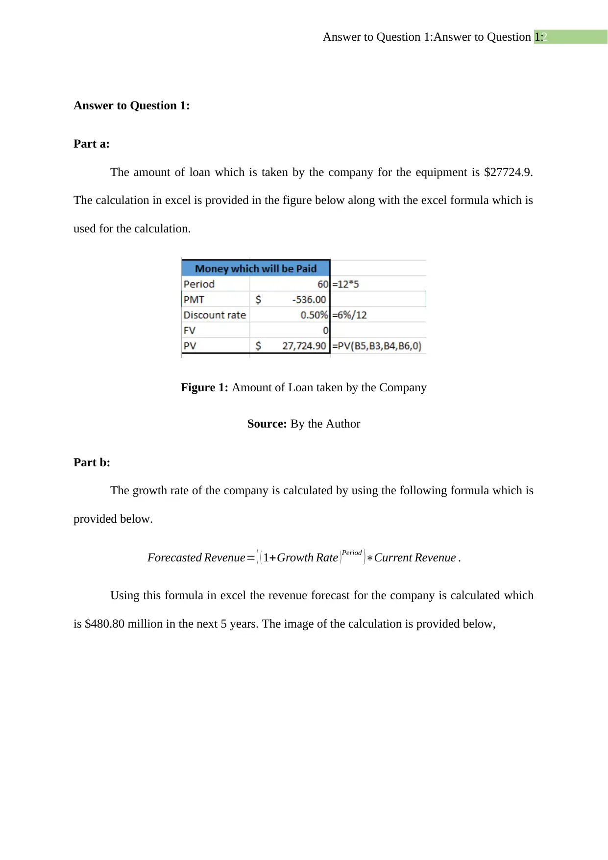
The amount of loan which is taken by the company for the equipment is $27724.9.
The calculation in excel is provided in the figure below along with the excel formula which is
used for the calculation.
Figure 1: Amount of Loan taken by the Company
Source: By the Author
Part b:
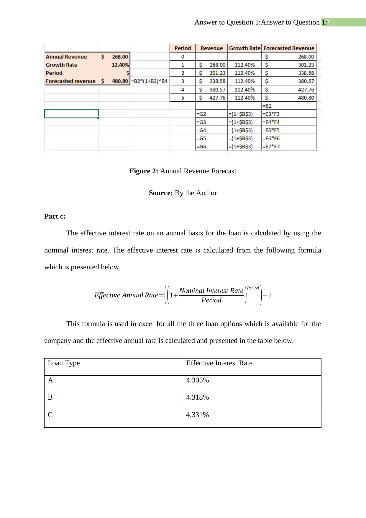
The growth rate of the company is calculated by using the following formula which is
provided below.
Forecasted Revenue= ( ( 1+Growth Rate ) Period )∗Current Revenue .
Using this formula in excel the revenue forecast for the company is calculated which
is $480.80 million in the next 5 years. The image of the calculation is provided below,
Answer to Question 1:
Part a:
The amount of loan which is taken by the company for the equipment is $27724.9.
The calculation in excel is provided in the figure below along with the excel formula which is
used for the calculation.
Figure 1: Amount of Loan taken by the Company
Source: By the Author
Part b:
The growth rate of the company is calculated by using the following formula which is
provided below.
Forecasted Revenue= ( ( 1+Growth Rate ) Period )∗Current Revenue .
Using this formula in excel the revenue forecast for the company is calculated which
is $480.80 million in the next 5 years. The image of the calculation is provided below,
⊘ This is a preview!⊘
Do you want full access?
Subscribe today to unlock all pages.
Trusted by 1+ million students worldwide
3Answer to Question 1:Answer to Question 1:
Figure 2: Annual Revenue Forecast
Source: By the Author
Part c:
The effective interest rate on an annual basis for the loan is calculated by using the
nominal interest rate. The effective interest rate is calculated from the following formula
which is presented below,
Effective Annual Rate=
( (1+ Nominal Interest Rate
Period )Period
)−1
This formula is used in excel for all the three loan options which is available for the
company and the effective annual rate is calculated and presented in the table below,
Loan Type Effective Interest Rate
A 4.305%
B 4.318%
C 4.331%
Paraphrase This Document
Need a fresh take? Get an instant paraphrase of this document with our AI Paraphraser
4Answer to Question 1:Answer to Question 1:
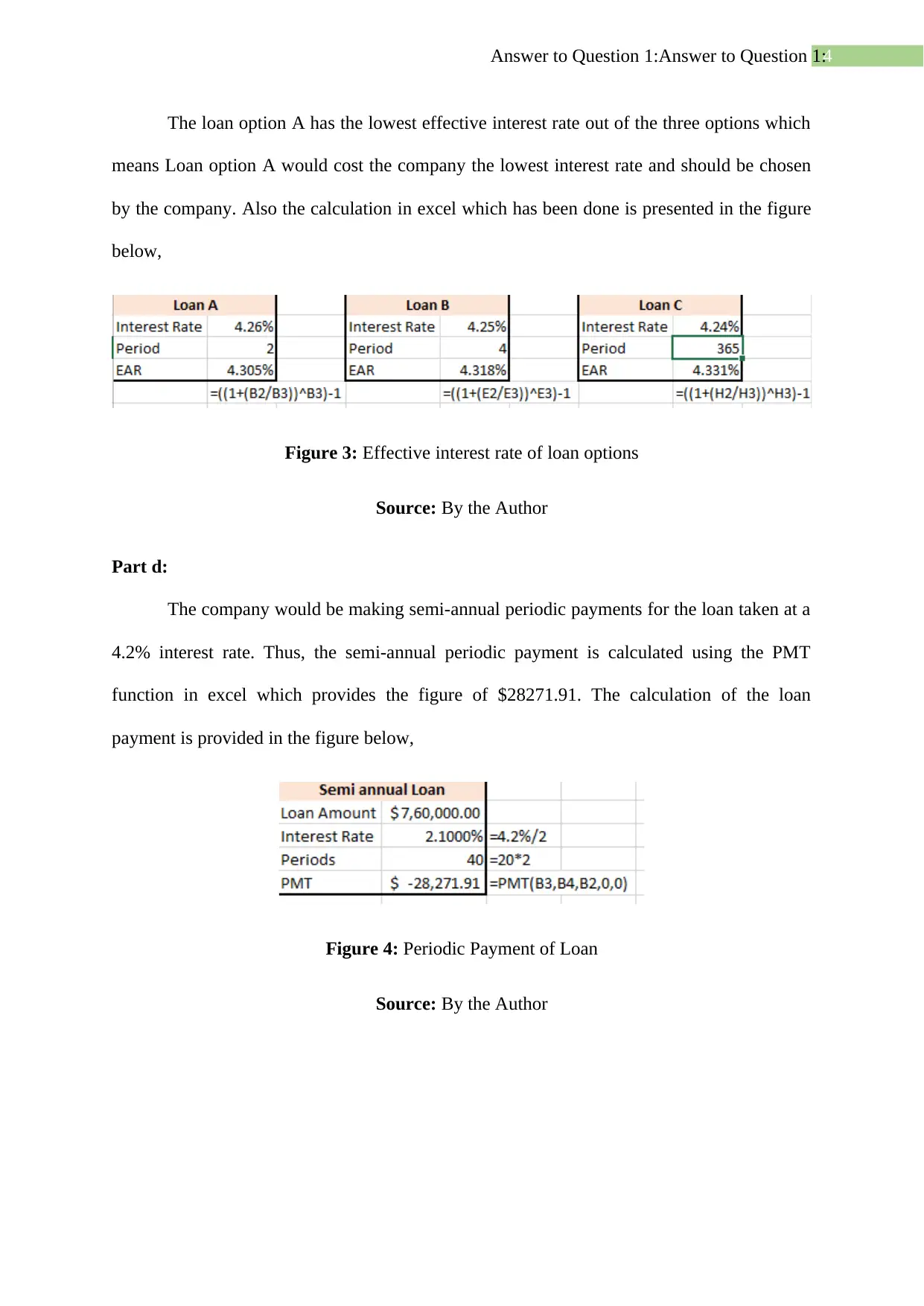
The loan option A has the lowest effective interest rate out of the three options which
means Loan option A would cost the company the lowest interest rate and should be chosen
by the company. Also the calculation in excel which has been done is presented in the figure
below,
Figure 3: Effective interest rate of loan options
Source: By the Author
Part d:
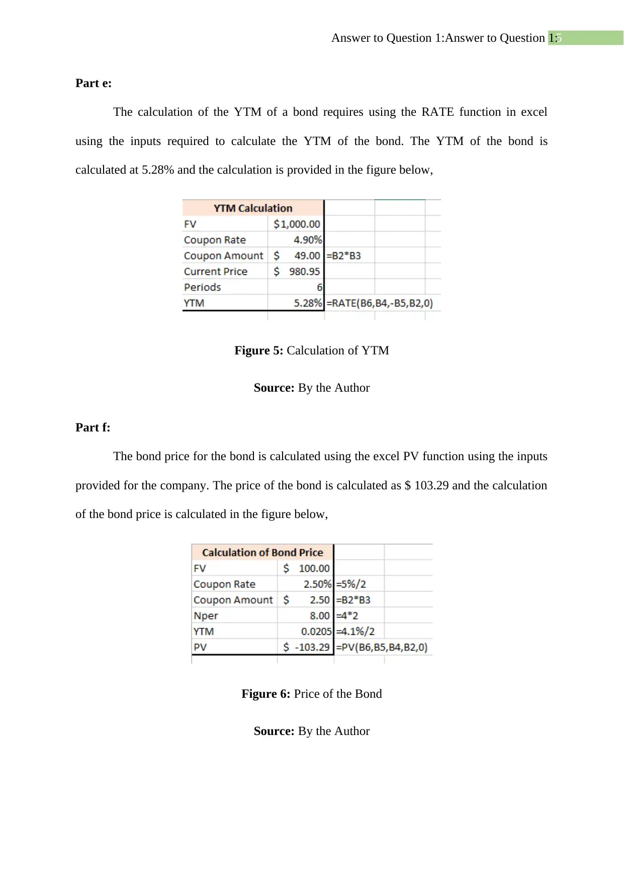
The company would be making semi-annual periodic payments for the loan taken at a
4.2% interest rate. Thus, the semi-annual periodic payment is calculated using the PMT
function in excel which provides the figure of $28271.91. The calculation of the loan
payment is provided in the figure below,
Figure 4: Periodic Payment of Loan
Source: By the Author
The loan option A has the lowest effective interest rate out of the three options which
means Loan option A would cost the company the lowest interest rate and should be chosen
by the company. Also the calculation in excel which has been done is presented in the figure
below,
Figure 3: Effective interest rate of loan options
Source: By the Author
Part d:
The company would be making semi-annual periodic payments for the loan taken at a
4.2% interest rate. Thus, the semi-annual periodic payment is calculated using the PMT
function in excel which provides the figure of $28271.91. The calculation of the loan
payment is provided in the figure below,
Figure 4: Periodic Payment of Loan
Source: By the Author
5Answer to Question 1:Answer to Question 1:
Part e:
The calculation of the YTM of a bond requires using the RATE function in excel
using the inputs required to calculate the YTM of the bond. The YTM of the bond is
calculated at 5.28% and the calculation is provided in the figure below,
Figure 5: Calculation of YTM
Source: By the Author
Part f:
The bond price for the bond is calculated using the excel PV function using the inputs
provided for the company. The price of the bond is calculated as $ 103.29 and the calculation
of the bond price is calculated in the figure below,
Figure 6: Price of the Bond
Source: By the Author
⊘ This is a preview!⊘
Do you want full access?
Subscribe today to unlock all pages.
Trusted by 1+ million students worldwide
6Answer to Question 1:Answer to Question 1:
Answer to Question 2:
Part a:
The expected return for the company Nick Scali Limited is calculated first by using
the historical stock price of the company. This is used to calculate the historical return of the
stock on a daily basis. The price of the index which is All Ordinaries is also taken for the
purpose of the calculation for calculating Beta.
The beta is a measurement of risk of the company which is calculated by regressing
the stock return over the market return. Thus, the Beta for the company Nick Scali is
calculated as 0.49. The risk free rate is taken as 0.9% which is the yield of 10 year Australian
Government bond as on 1st April 2020. The market risk premium is provided as 5.5%. The
market risk premium is assumed to be given by Return of the market less the Risk free Rate.
The expected return for the stock is calculated using the formula of CAPM which is provided
below,
Expected Return=Risk Free Rate+ ( Rm−Rf )∗Beta
The expected Return for the case company is calculated in the following steps using
the inputs,
Risk Free Rate – 0.9%
Market Return – 5.5%
Beta – 0.49
Expected Return=0.9 %+ ( 5.5 %−0.9% )∗0.49
Expected Return=0.9 %+ ( 4.6 % )∗0.49
Expected Return=0.9 %+2.27 %=3.17 %
Paraphrase This Document
Need a fresh take? Get an instant paraphrase of this document with our AI Paraphraser
7Answer to Question 1:Answer to Question 1:
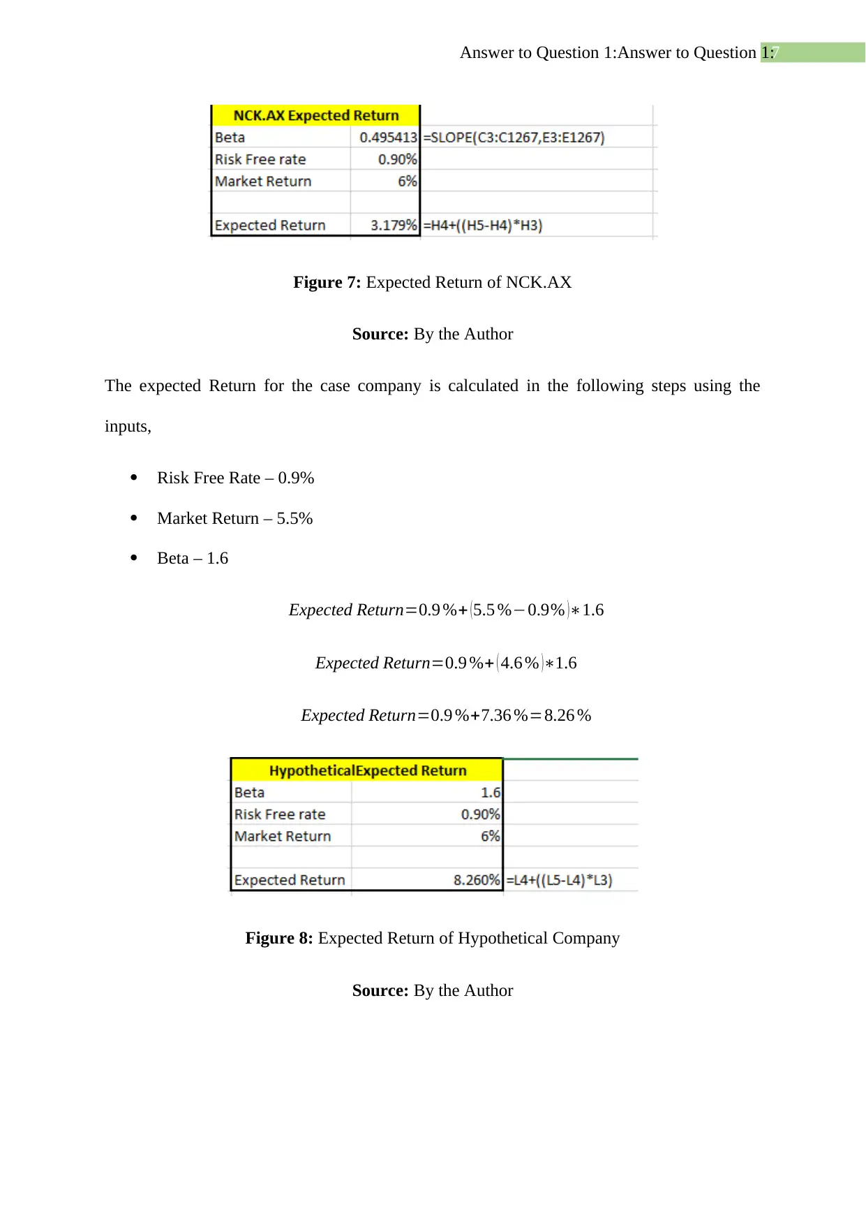
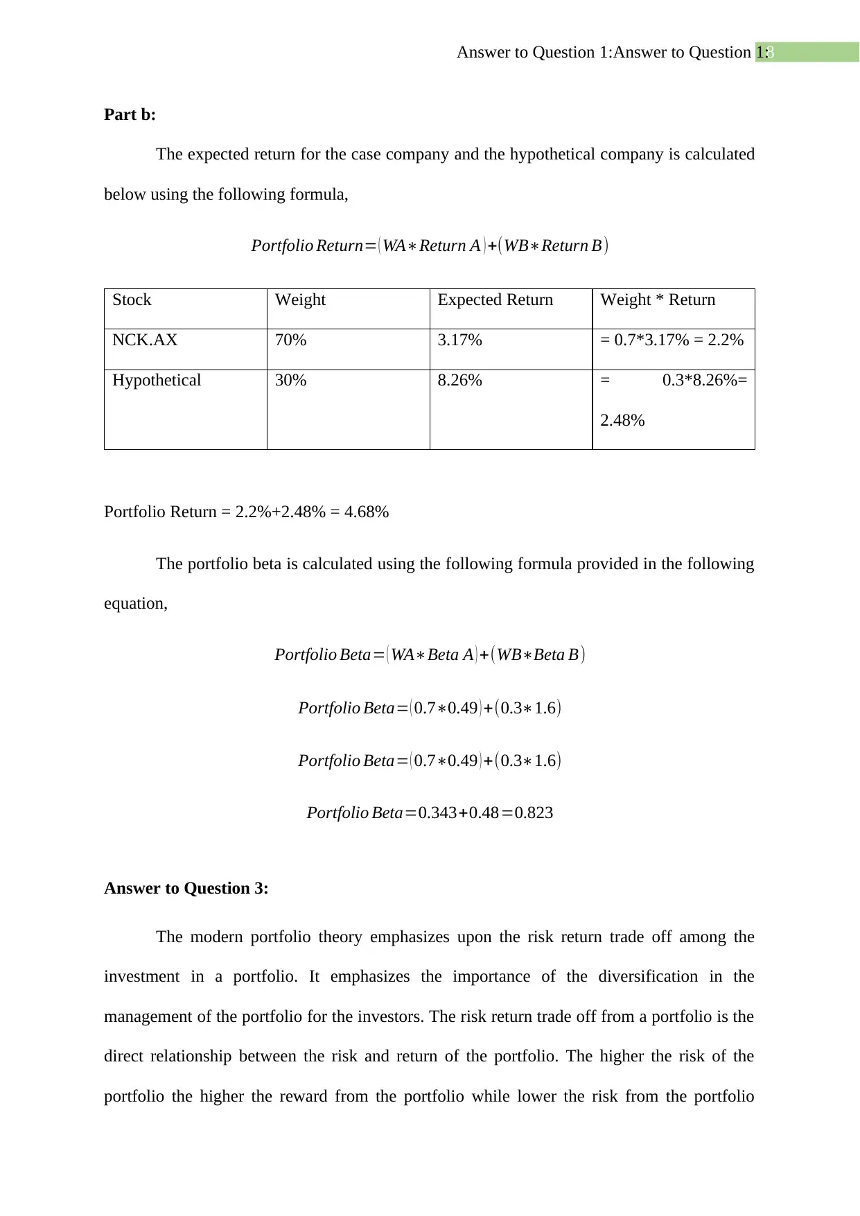
Figure 7: Expected Return of NCK.AX
Source: By the Author
The expected Return for the case company is calculated in the following steps using the
inputs,
Risk Free Rate – 0.9%
Market Return – 5.5%
Beta – 1.6
Expected Return=0.9 %+ (5.5 %−0.9% )∗1.6
Expected Return=0.9 %+ ( 4.6 % )∗1.6
Expected Return=0.9 %+7.36 %=8.26 %
Figure 8: Expected Return of Hypothetical Company
Source: By the Author
8Answer to Question 1:Answer to Question 1:
Part b:
The expected return for the case company and the hypothetical company is calculated
below using the following formula,
Portfolio Return= ( WA∗Return A ) +(WB∗Return B)
Stock Weight Expected Return Weight * Return
NCK.AX 70% 3.17% = 0.7*3.17% = 2.2%
Hypothetical 30% 8.26% = 0.3*8.26%=
2.48%
Portfolio Return = 2.2%+2.48% = 4.68%
The portfolio beta is calculated using the following formula provided in the following
equation,
Portfolio Beta= ( WA∗Beta A ) +(WB∗Beta B)
Portfolio Beta= ( 0.7∗0.49 ) +(0.3∗1.6)
Portfolio Beta= ( 0.7∗0.49 ) +(0.3∗1.6)
Portfolio Beta=0.343+0.48=0.823
Answer to Question 3:
The modern portfolio theory emphasizes upon the risk return trade off among the
investment in a portfolio. It emphasizes the importance of the diversification in the
management of the portfolio for the investors. The risk return trade off from a portfolio is the
direct relationship between the risk and return of the portfolio. The higher the risk of the
portfolio the higher the reward from the portfolio while lower the risk from the portfolio
⊘ This is a preview!⊘
Do you want full access?
Subscribe today to unlock all pages.
Trusted by 1+ million students worldwide
9Answer to Question 1:Answer to Question 1:
lower the return. This can be understood by the empirical example between bonds and equity,
where bonds are considered relatively less risky than equity. Thus the return which is
required by the debt providers of the company is less than the equity providers since the debt
is covered by the assets of the company (Chandra 2017).
Thus, as per empirical theory between the risk return trade off, higher the risk higher
the return required by the investors. Here the importance of diversification benefit arises in
the portfolio, where the unsystematic risk from the portfolio is reduced while the investors
are rewarded for the systematic risk. The unsystematic risk implies the risk which is only
faced by a particular company and not the overall market, while systematic risk implies the
risk which affects the overall market. The investor can diversify the portfolio which means
reducing or eliminating the unsystematic risk from the portfolio (Antchak, Ziakas and Getz
2019).
The elimination of the unsystematic risk depends on the correlation between the asset
class and also upon the correlation among the investment in the asset class. The correlation
between the bond and the equity asset class is low which has been observed during the
market crashes. As when the market crashes the price of equity falls while debt rises which
implies a negative correlation among the asset class. Thus, when the economy is expected to
boom, the manager can increases the level of equity in a portfolio while reduce the level of
debt since equity performs well in economic boom generating higher return. Also when the
investments with in the asset class have lower correlation the benefits of diversification is
higher in the portfolio. This reduces the unsystematic risk or diversifiable risk from the
portfolio and the investor is awarded for the systematic risk.
Based on this knowledge the company Nick Scali which has a beta of 0.49 while an
expected return of 3.17% and the hypothetical company has beta of 1.6 and a return of
Paraphrase This Document
Need a fresh take? Get an instant paraphrase of this document with our AI Paraphraser
10Answer to Question 1:Answer to Question 1:
8.26%. This highlights the direct relationship between risk return of the portfolio. The Beta of
the portfolio is 0.82 while the expected return is 4.7%. The investor has been able to increase
the risk of the investment along with the return as per the risk tolerance level. However, the
portfolio constructed cannot be defined as the optimal portfolio for the investor. The optimal
portfolio factors in the available various set of opportunity of the portfolio investment which
is available for the investor and constructs the portfolio which provides the highest level of
return for the least level of risk (Nawrocka 2018).
The optimal portfolio for investment is constructed using the Markowitz efficient
frontier curve, which is a curve consisting of various risk and return level for the portfolio.
The capital allocation line is also constructed using the market portfolio and the risk free rate
of investment. The optimal portfolio or the portfolio which maximizes the return while
reducing the risk is a tangent with the capital allocation line. This portfolio should be selected
by a rational investor as it reduces the unsystematic risk to the maximum level,
The Beta is a measure to analyse the risk of the investment as it measures the risk
with respect to the market portfolio. The market portfolio is assumed to be the diversified
portfolio which has a beta which is equal to 1. A beta measure less than 1 implies a less risky
investment and more than 1 implies high risk investment. The NCK.AX stock is a low risk
investment which provides a lower return which is increased when invested in the portfolio.
The hypothetical company is a high risk investment which is reduced in the portfolio. Thus
the correlation is one of the most important determinants which provides diversification to
the portfolio. Higher the correlation the lower the diversification benefit while lower the
correlation the higher the diversification benefit (Alford, Luchtenberg and Reddie 2018).
11Answer to Question 1:Answer to Question 1:
References:
Alford, R.M., Luchtenberg, K.F. and Reddie, W.D., 2018. Portfolio Management and
Earnings Management: Evidence from Property and Casualty Insurers. Journal of
Accounting & Finance (2158-3625), 18(4).
Antchak, V., Ziakas, V. and Getz, D., 2019. Event portfolio management: theory and
methods for event management and tourism. Goodfellow.
Bloomberg - Are you a robot? (2020). Available at:
https://www.bloomberg.com/markets/rates-bonds/government-bonds/australia (Accessed: 13
April 2020).
Chakrabarty, R., Roy, T. and Chaudhuri, K.S., 2017. A production: inventory model for
defective items with shortages incorporating inflation and time value of money. International
Journal of Applied and Computational Mathematics, 3(1), pp.195-212.
Chandra, P., 2017. Investment analysis and portfolio management. McGraw-hill education.
Dong, J., Korobenko, L. and Deniz Sezer, A., 2020. A variation of Merton's corporate bond
valuation model for firms with illiquid but observable assets. Quantitative Finance, 20(3),
pp.483-497.
García-Schmidt, M. and Woodford, M., 2019. Are low interest rates deflationary? A paradox
of perfect-foresight analysis. American Economic Review, 109(1), pp.86-120.
Kahn, M.J. and Baum, N., 2020. Time Value of Money, or What Is the Real Financial Value
of an Opportunity?. In The Business Basics of Building and Managing a Healthcare
Practice (pp. 9-12). Springer, Cham.
⊘ This is a preview!⊘
Do you want full access?
Subscribe today to unlock all pages.
Trusted by 1+ million students worldwide
1 out of 13
Related Documents


Your All-in-One AI-Powered Toolkit for Academic Success.
+13062052269
info@desklib.com
Available 24*7 on WhatsApp / Email
![[object Object]](/_next/static/media/star-bottom.7253800d.svg)
Unlock your academic potential
Copyright © 2020–2026 A2Z Services. All Rights Reserved. Developed and managed by ZUCOL.