Statistical Analysis of Business and Finance Data Assignment

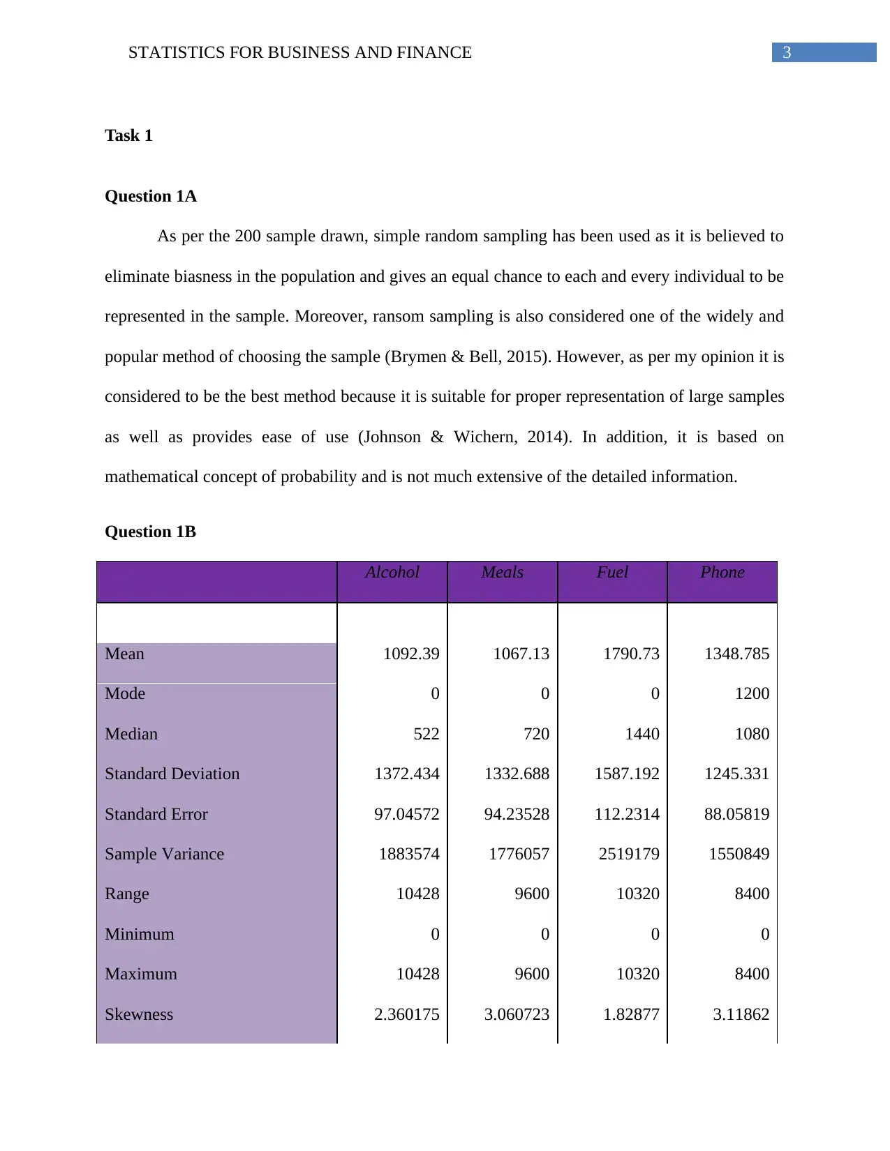
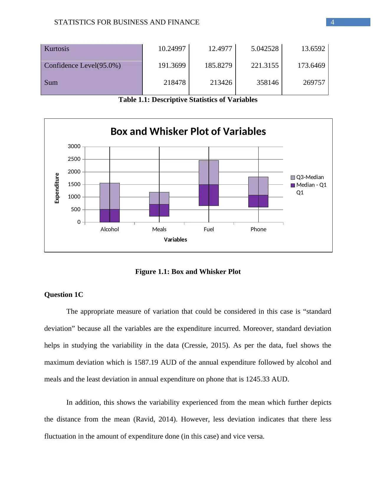
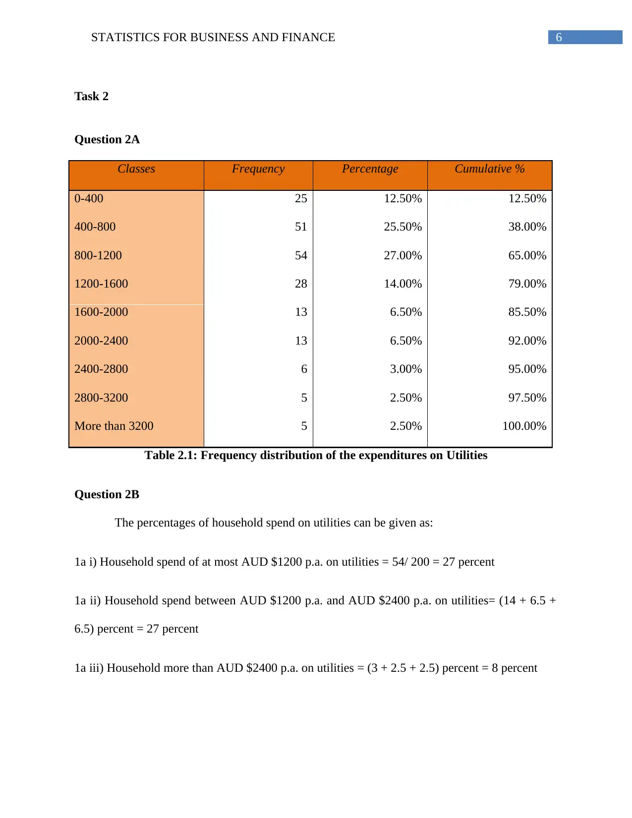
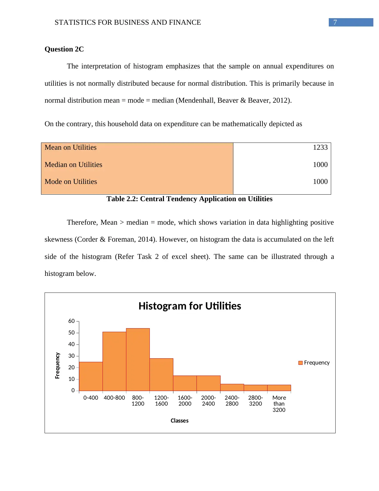
This statistics assignment analyzes business and finance data using various statistical methods. It begins with descriptive statistics, including measures of central tendency, variation, and data distribution, examining variables like alcohol, meals, fuel, and phone expenditures. The assignment then delves into frequency distributions and histograms to analyze utility expenditures, exploring concepts like normal distribution and skewness. Further, the solution addresses percentiles, probabilities related to household characteristics (home ownership, family size), and correlations between after-tax income and total expenditure using scatter plots. Finally, the assignment uses contingency tables to explore the relationship between gender and education level, calculating conditional probabilities and determining the independence of variables related to gender and education.

Running head: STATISTICS FOR BUSINESS AND FINANCE
Statistics for Business and Finance
Name of the student:
Name of the university:
Authors note:

1STATISTICS FOR BUSINESS AND FINANCE
Table of Contents
Task 1...............................................................................................................................................3
Question 1A.................................................................................................................................3
Question 1B.................................................................................................................................3
Question 1C.................................................................................................................................4
Question 1D.................................................................................................................................5
Task 2...............................................................................................................................................6
Question 2A.................................................................................................................................6
Question 2B.................................................................................................................................6
Question 2C.................................................................................................................................7
Task 3...............................................................................................................................................8
Question 3A.................................................................................................................................8
Question 3B.................................................................................................................................8
Question 3C.................................................................................................................................8
Question 3D.................................................................................................................................8
Task 4.............................................................................................................................................10
Question 4A...............................................................................................................................10
Question 4B...............................................................................................................................10
Question 4C...............................................................................................................................11

2STATISTICS FOR BUSINESS AND FINANCE
Question 4D...............................................................................................................................11
Question 4E...............................................................................................................................11
References......................................................................................................................................13

3STATISTICS FOR BUSINESS AND FINANCE
Task 1
Question 1A
As per the 200 sample drawn, simple random sampling has been used as it is believed to
eliminate biasness in the population and gives an equal chance to each and every individual to be
represented in the sample. Moreover, ransom sampling is also considered one of the widely and
popular method of choosing the sample (Brymen & Bell, 2015). However, as per my opinion it is
considered to be the best method because it is suitable for proper representation of large samples
as well as provides ease of use (Johnson & Wichern, 2014). In addition, it is based on
mathematical concept of probability and is not much extensive of the detailed information.
Question 1B
Alcohol Meals Fuel Phone
Mean 1092.39 1067.13 1790.73 1348.785
Mode 0 0 0 1200
Median 522 720 1440 1080
Standard Deviation 1372.434 1332.688 1587.192 1245.331
Standard Error 97.04572 94.23528 112.2314 88.05819
Sample Variance 1883574 1776057 2519179 1550849
Range 10428 9600 10320 8400
Minimum 0 0 0 0
Maximum 10428 9600 10320 8400
Skewness 2.360175 3.060723 1.82877 3.11862

4STATISTICS FOR BUSINESS AND FINANCE
Kurtosis 10.24997 12.4977 5.042528 13.6592
Confidence Level(95.0%) 191.3699 185.8279 221.3155 173.6469
Sum 218478 213426 358146 269757
Table 1.1: Descriptive Statistics of Variables
Alcohol Meals Fuel Phone
0
500
1000
1500
2000
2500
3000
Box and Whisker Plot of Variables
Q3-Median
Median - Q1
Q1
Variables
Expenditure
Figure 1.1: Box and Whisker Plot
Question 1C
The appropriate measure of variation that could be considered in this case is “standard
deviation” because all the variables are the expenditure incurred. Moreover, standard deviation
helps in studying the variability in the data (Cressie, 2015). As per the data, fuel shows the
maximum deviation which is 1587.19 AUD of the annual expenditure followed by alcohol and
meals and the least deviation in annual expenditure on phone that is 1245.33 AUD.
In addition, this shows the variability experienced from the mean which further depicts
the distance from the mean (Ravid, 2014). However, less deviation indicates that there less
fluctuation in the amount of expenditure done (in this case) and vice versa.

5STATISTICS FOR BUSINESS AND FINANCE
Question 1D
The box plots as given part 2 of the question highlights that the variability is maximum in
fuels followed by alcohol from the upper quartile and median. Moreover, as per the expenditure
on the data distribution, the data has been shown to be less in lower quartile than in upper
quartile (Hahs-Vaughn & Lomax, 2013). Also, through descriptive statistics, for all the four
variables that is alcohol, meals, fuels and phone, the mean >median >mode. This depicts the data
is slightly higher in the end tail (positive skewed / upper quartile of box plot). Conversely, it
underlines annual expenditure on these four highlighted variables is high.

6STATISTICS FOR BUSINESS AND FINANCE
Task 2
Question 2A
Classes Frequency Percentage Cumulative %
0-400 25 12.50% 12.50%
400-800 51 25.50% 38.00%
800-1200 54 27.00% 65.00%
1200-1600 28 14.00% 79.00%
1600-2000 13 6.50% 85.50%
2000-2400 13 6.50% 92.00%
2400-2800 6 3.00% 95.00%
2800-3200 5 2.50% 97.50%
More than 3200 5 2.50% 100.00%
Table 2.1: Frequency distribution of the expenditures on Utilities
Question 2B
The percentages of household spend on utilities can be given as:
1a i) Household spend of at most AUD $1200 p.a. on utilities = 54/ 200 = 27 percent
1a ii) Household spend between AUD $1200 p.a. and AUD $2400 p.a. on utilities= (14 + 6.5 +
6.5) percent = 27 percent
1a iii) Household more than AUD $2400 p.a. on utilities = (3 + 2.5 + 2.5) percent = 8 percent

7STATISTICS FOR BUSINESS AND FINANCE
Question 2C
The interpretation of histogram emphasizes that the sample on annual expenditures on
utilities is not normally distributed because for normal distribution. This is primarily because in
normal distribution mean = mode = median (Mendenhall, Beaver & Beaver, 2012).
On the contrary, this household data on expenditure can be mathematically depicted as
Mean on Utilities 1233
Median on Utilities 1000
Mode on Utilities 1000
Table 2.2: Central Tendency Application on Utilities
Therefore, Mean > median = mode, which shows variation in data highlighting positive
skewness (Corder & Foreman, 2014). However, on histogram the data is accumulated on the left
side of the histogram (Refer Task 2 of excel sheet). The same can be illustrated through a
histogram below.
0-400 400-800 800-
1200 1200-
1600 1600-
2000 2000-
2400 2400-
2800 2800-
3200 More
than
3200
0
10
20
30
40
50
60
Histogram for Utilities
Frequency
Classes
Frequency

8STATISTICS FOR BUSINESS AND FINANCE
Figure 2.1: Histogram on Utilities
Task 3
Question 3A
Values of ATaxInc calculated and percentile method has been applied (Refer Task 3 of
excel sheet).
 Lower 10th Percentile =PERCENTILE(K2:K201,0.1) = 1575.6
Upper 10th Percentile =PERCENTILE(K2:K201,0.9) = 10307.9
Question 3B
The number of household that have their own house = 135
Mean of own house = 135/ 200 = 0.68
As per the average implies, there are more than average number of households that own a house.
Question 3C
The number of family size (adults + children) = 13
“=COUNTIF (C2:C201,"= 5")” (Excel)
Probability of “Family size =5” =0.065
Question 3D
The ln(texp) against ln(ataxinc) is explained using a scatter lot as shown below in Figure
3.1. Moreover, the scatter is in form of upload sloping and scattered at one place only. Also, the
correlation between the log of after tax annual income and total expenditure is r = 0.994513

9STATISTICS FOR BUSINESS AND FINANCE
highlighting the relationship between both the variables is high as the r is between 0.5 and 1
which shows strong and positive correlation.
7.500
8.000
8.500
9.000
9.500
10.000
10.500
11.000
11.500
0.000
2.000
4.000
6.000
8.000
10.000
12.000
14.000
Relationship of two variables
Relationship of two variables
Ln (Atexp)
Ln (ATaxInc)
Figure 3.1: Scatter Plot of Ln(ATaxInc) and Ln(Atexp)

10STATISTICS FOR BUSINESS AND FINANCE
Task 4
Question 4A
Highest Degree\ Gender Female Male
Bachelor 20 15
Intermediate 18 32
Master 15 16
Primary 16 23
Secondary 23 22
Total 92 108
Table 4.1: Contingency Table
The contingency table explains that higher education for the males as well as females.
The higher level of education accompanies bachelor’s degree and master’s degree. However, as
per the data females count is (15+20) 35 whereas for males is (16+15) 31. This depicts that
households have stark contrast in higher level of education amongst the males and females.
Question 4B
Highest Degree\ Gender Female Male Total
Bachelor 0.100 0.075 0.175
Intermediate 0.090 0.160 0.250
Master 0.075 0.080 0.155
Primary 0.080 0.115 0.195
Secondary 0.115 0.110 0.225

11STATISTICS FOR BUSINESS AND FINANCE
Total 0.460 0.540 1.000
Pr (Female as head of household and Intermediate level of
education)
(Female and Intermediate/ Total
Sample)
18/200 = 0.09 9%
Question 4C
Pr (Male as head of household and Bachelors level of
education)
(Male and Bachelors/ Total
Sample)
16/200 = 0.080 8%
Question 4D
Pr (Secondary Degree as among females) (Secondary Degree among females/ Total females)
23/92 = 0.250 25%
Question 4E
Pr (A= Gender as Male) 108/200 = 0.65 54%
Pr (B = Level of Education as Master’s Degree) 31/200 = 0.1 15.5%
Pr (A) * Pr (B) 0.54*0.155 =
0.0837
8.37%
Pr (AB) 16/200 = 0.080 8%
 It can be seen that Pr (A)*Pr (B) ≠ Pr (AB)