BBA 315 Business Forecasting: Visitors Arrival Trend Analysis

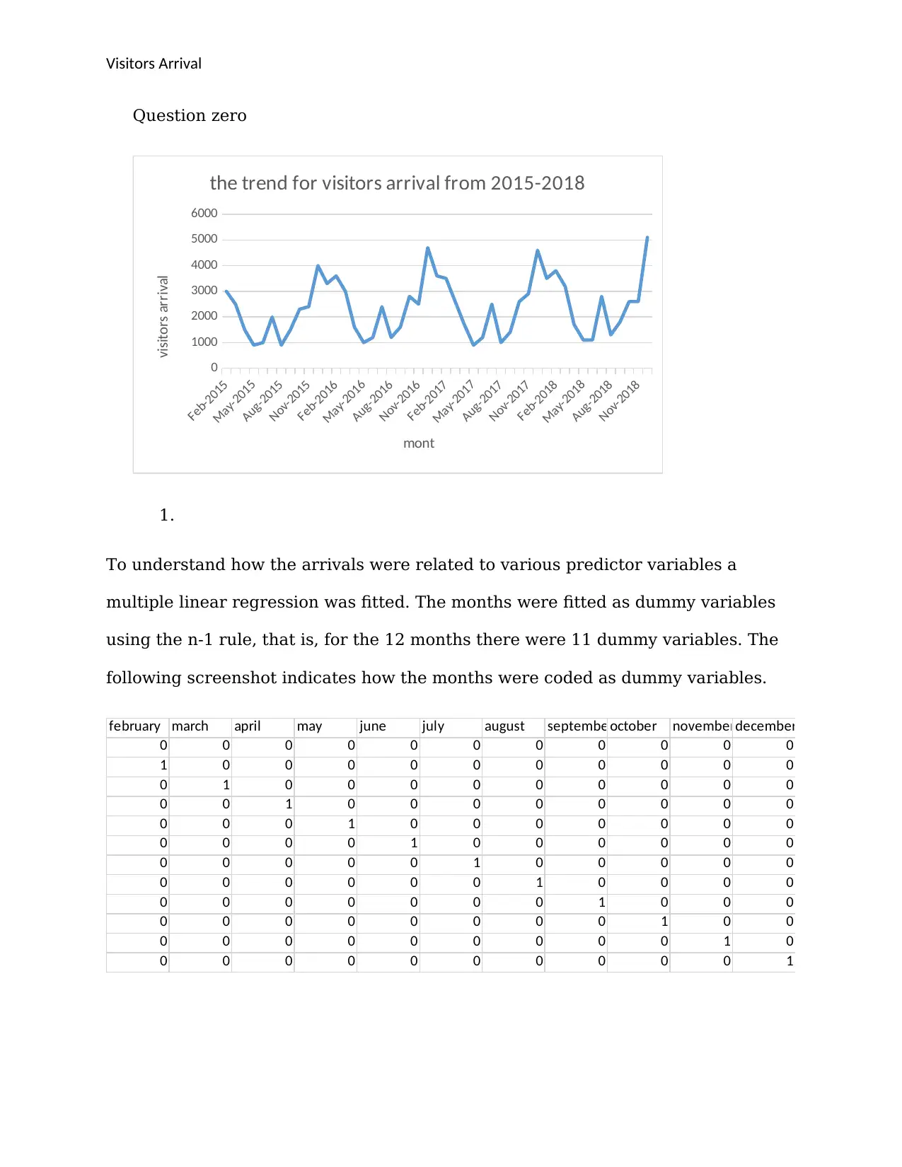
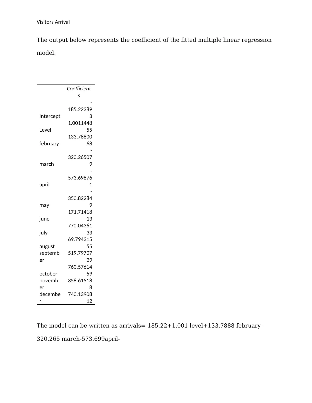
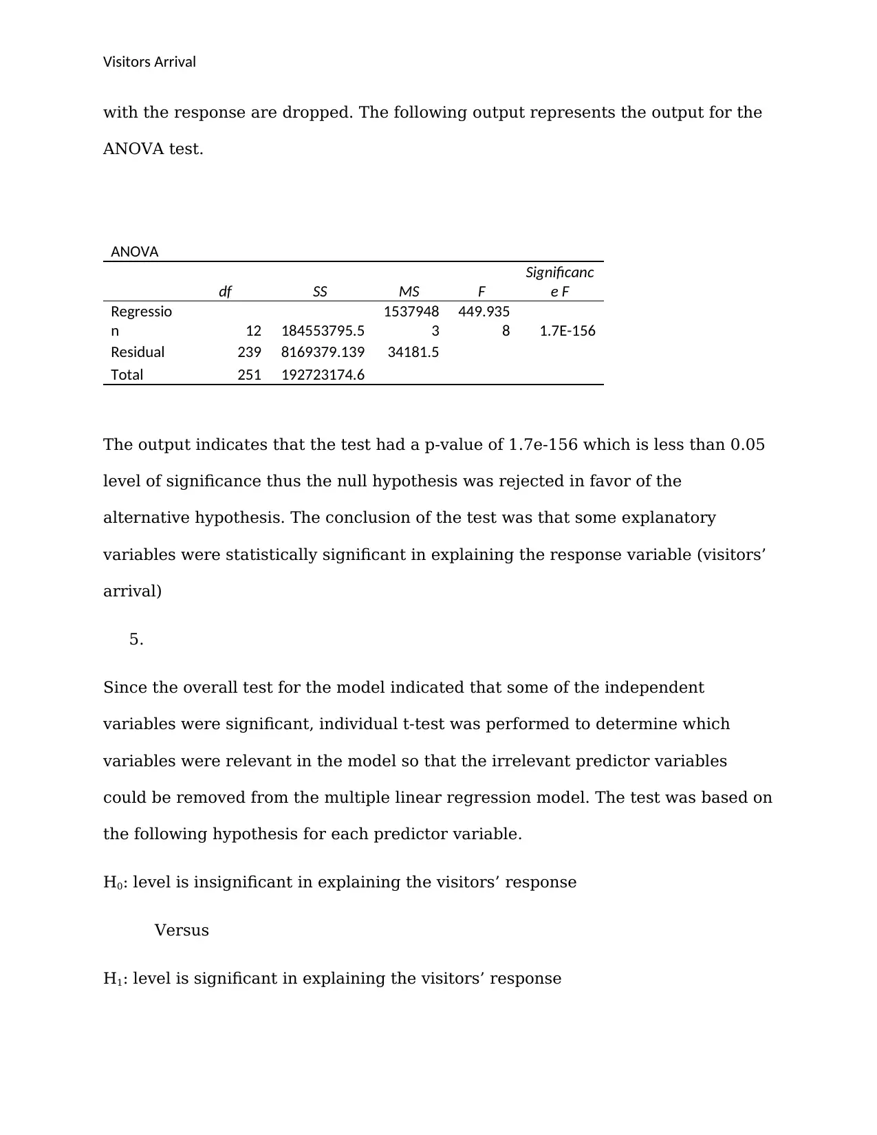
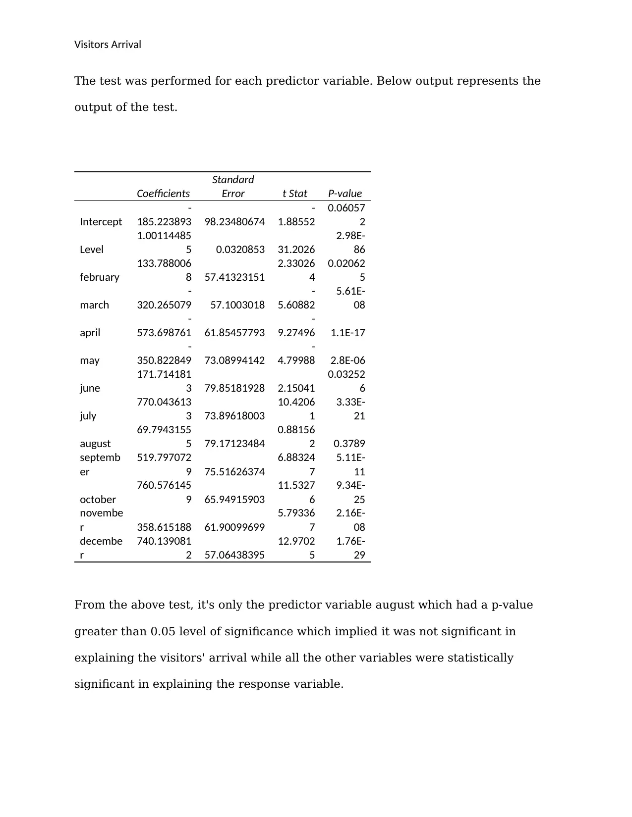
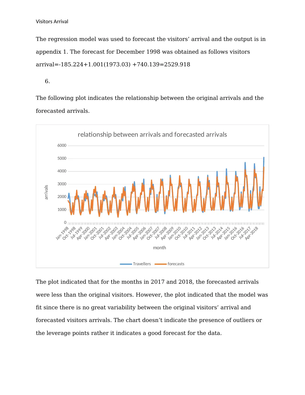
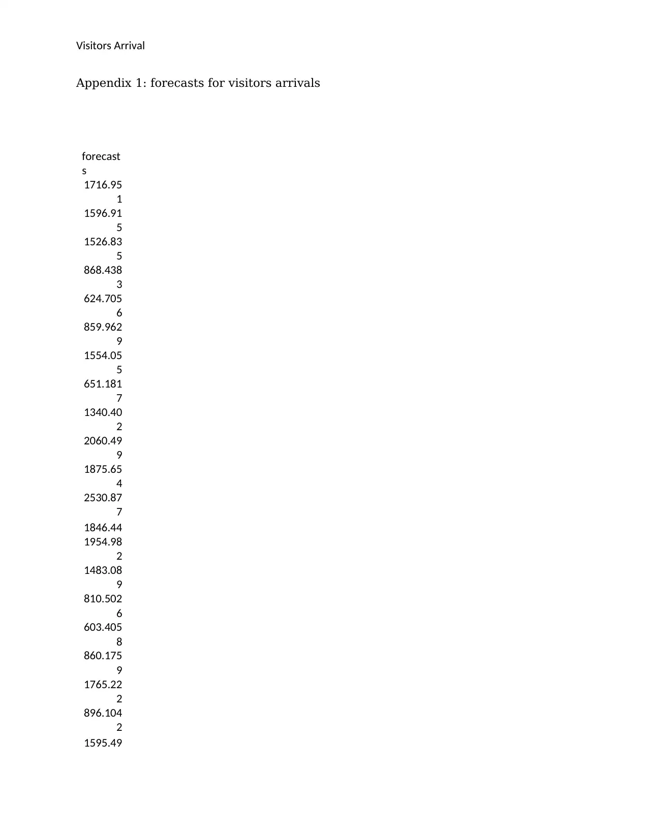
This case study report focuses on analyzing visitor arrival trends from 2015 to 2018 using business forecasting techniques. A multiple linear regression model was fitted to understand how arrivals relate to predictor variables, including monthly dummy variables. The model's coefficients, R-squared value (97.86%), and ANOVA results are presented, indicating the significance of explanatory variables. Individual t-tests were performed to determine variable relevance, leading to a reduced model focusing on March, June, September, and December. The regression model was used to forecast visitor arrivals, and the relationship between original and forecasted arrivals is visually represented. The analysis includes a forecast for December 1998 and concludes that while some forecasted arrivals were less than original values, the model generally fits the data well. Appendix 1 provides detailed forecasts for visitor arrivals.

Visitors Arrival
Question zero
Feb-2015
May-2015
Aug-2015
Nov-2015
Feb-2016
May-2016
Aug-2016
Nov-2016
Feb-2017
May-2017
Aug-2017
Nov-2017
Feb-2018
May-2018
Aug-2018
Nov-2018
0
1000
2000
3000
4000
5000
6000
the trend for visitors arrival from 2015-2018
mont
visitors arrival
1.
To understand how the arrivals were related to various predictor variables a
multiple linear regression was fitted. The months were fitted as dummy variables
using the n-1 rule, that is, for the 12 months there were 11 dummy variables. The
following screenshot indicates how the months were coded as dummy variables.
february march april may june july august septemberoctober novemberdecember
0 0 0 0 0 0 0 0 0 0 0
1 0 0 0 0 0 0 0 0 0 0
0 1 0 0 0 0 0 0 0 0 0
0 0 1 0 0 0 0 0 0 0 0
0 0 0 1 0 0 0 0 0 0 0
0 0 0 0 1 0 0 0 0 0 0
0 0 0 0 0 1 0 0 0 0 0
0 0 0 0 0 0 1 0 0 0 0
0 0 0 0 0 0 0 1 0 0 0
0 0 0 0 0 0 0 0 1 0 0
0 0 0 0 0 0 0 0 0 1 0
0 0 0 0 0 0 0 0 0 0 1

Visitors Arrival
The output below represents the coefficient of the fitted multiple linear regression
model.
Coefficient
s
Intercept
-
185.22389
3
Level
1.0011448
55
february
133.78800
68
march
-
320.26507
9
april
-
573.69876
1
may
-
350.82284
9
june
171.71418
13
july
770.04361
33
august
69.794315
55
septemb
er
519.79707
29
october
760.57614
59
novemb
er
358.61518
8
decembe
r
740.13908
12
The model can be written as arrivals=-185.22+1.001 level+133.7888 february-
320.265 march-573.699april-

Visitors Arrival
350.822may+171.714june+770.044july+69.794august+519.797september+760.5
76october+358.615november+740.139december.
1.
The intercept indicates that when each of the predictor variables is zero the
average visitors' arrival is 185.22. The coefficient for the level showed that the
visitors' arrival increase by 1.001 units per unit increase in the levels holding other
predictor variables constant. The coefficient for June indicates that the visitors'
arrival for June was 171.714 more than the visitors' arrival for January holding
other predictor variables constant.
2.
The fitted model had R-square of 97.86%. R-squared indicates the variability of the
model that is explained by predictor variables in the model. The R-squared for this
model indicated that 97.86% variability of the model was explained by the
explanatory variables in the model while only 2.14% of the variability was
explained by other factors, not in the model. R-squared is important in assessing
the accuracy of the model, that is, how well the model fits the data. Heuristically,
when the value of R-squared is close to 1 it indicates the model perfectly fit the
data while the value of R-squared close to zero indicates that the model is poor for
the data. For the model above R-squared was 97.86 which is close to one, this
indicated that the model perfectly fits the data.
3.
The following model represents the reduced model for March, June, September,
and December.

Visitors Arrival
Arrivals=1889.286+329.762march-851.9june-
303.571September+1429.762December
The following charts indicate the above model.
0 2 4 6 8 10 12
0
2
4
6
8
10
12
forecast
4.
To investigate whether the explanatory variables are significant in explaining the
visitors’ arrival, analysis of variance (ANOVA) was performed at 5% level of
significance. The test was based on the following hypothesis.
H0: the predictor variables are insignificant in explaining the visitors’ arrival
Versus
H1: some predictor variables are significant in explaining the visitors’ arrival
The test helps in determining whether the independent variables are associated
with the response variable. If the null hypothesis is rejected a test to determine
which predictor variables are significant is performed. Variables not associated

Visitors Arrival
with the response are dropped. The following output represents the output for the
ANOVA test.
ANOVA
df SS MS F
Significanc
e F
Regressio
n 12 184553795.5
1537948
3
449.935
8 1.7E-156
Residual 239 8169379.139 34181.5
Total 251 192723174.6
The output indicates that the test had a p-value of 1.7e-156 which is less than 0.05
level of significance thus the null hypothesis was rejected in favor of the
alternative hypothesis. The conclusion of the test was that some explanatory
variables were statistically significant in explaining the response variable (visitors’
arrival)
5.
Since the overall test for the model indicated that some of the independent
variables were significant, individual t-test was performed to determine which
variables were relevant in the model so that the irrelevant predictor variables
could be removed from the multiple linear regression model. The test was based on
the following hypothesis for each predictor variable.
H0: level is insignificant in explaining the visitors’ response
Versus
H1: level is significant in explaining the visitors’ response

Visitors Arrival
The test was performed for each predictor variable. Below output represents the
output of the test.
Coefficients
Standard
Error t Stat P-value
Intercept
-
185.223893 98.23480674
-
1.88552
0.06057
2
Level
1.00114485
5 0.0320853 31.2026
2.98E-
86
february
133.788006
8 57.41323151
2.33026
4
0.02062
5
march
-
320.265079 57.1003018
-
5.60882
5.61E-
08
april
-
573.698761 61.85457793
-
9.27496 1.1E-17
may
-
350.822849 73.08994142
-
4.79988 2.8E-06
june
171.714181
3 79.85181928 2.15041
0.03252
6
july
770.043613
3 73.89618003
10.4206
1
3.33E-
21
august
69.7943155
5 79.17123484
0.88156
2 0.3789
septemb
er
519.797072
9 75.51626374
6.88324
7
5.11E-
11
october
760.576145
9 65.94915903
11.5327
6
9.34E-
25
novembe
r 358.615188 61.90099699
5.79336
7
2.16E-
08
decembe
r
740.139081
2 57.06438395
12.9702
5
1.76E-
29
From the above test, it's only the predictor variable august which had a p-value
greater than 0.05 level of significance which implied it was not significant in
explaining the visitors' arrival while all the other variables were statistically
significant in explaining the response variable.

Visitors Arrival
The regression model was used to forecast the visitors’ arrival and the output is in
appendix 1. The forecast for December 1998 was obtained as follows visitors
arrival=-185.224+1.001(1973.03) +740.139=2529.918
6.
The following plot indicates the relationship between the original arrivals and the
forecasted arrivals.
Jan-1998
Oct-1998
Jul-1999
Apr-2000
Jan-2001
Oct-2001
Jul-2002
Apr-2003
Jan-2004
Oct-2004
Jul-2005
Apr-2006
Jan-2007
Oct-2007
Jul-2008
Apr-2009
Jan-2010
Oct-2010
Jul-2011
Apr-2012
Jan-2013
Oct-2013
Jul-2014
Apr-2015
Jan-2016
Oct-2016
Jul-2017
Apr-2018
0
1000
2000
3000
4000
5000
6000
relationship between arrivals and forecasted arrivals
Travellers forecasts
month
arrivals
The plot indicated that for the months in 2017 and 2018, the forecasted arrivals
were less than the original visitors. However, the plot indicated that the model was
fit since there is no great variability between the original visitors’ arrival and
forecasted visitors arrivals. The chart doesn’t indicate the presence of outliers or
the leverage points rather it indicates a good forecast for the data.

Visitors Arrival
Appendix 1: forecasts for visitors arrivals
forecast
s
1716.95
1
1596.91
5
1526.83
5
868.438
3
624.705
6
859.962
9
1554.05
5
651.181
7
1340.40
2
2060.49
9
1875.65
4
2530.87
7
1846.44
1954.98
2
1483.08
9
810.502
6
603.405
8
860.175
9
1765.22
2
896.104
2
1595.49

Visitors Arrival
8
2262.39
5
1935.56
8
2495.79
6
1854.22
1
2048.10
1
1634.94
3
948.923
9
679.307
2
993.546
7
1787.18
4
944.165
4
1914.70
3
2609.22
2
2339.29
1
2827.36
3
2029.89
4
2169.53
4
1575.88
6
828.503
7
481.193
9
856.384
1751.12
8
828.916
9
1496.82
5

Visitors Arrival
2197.82
1897.72
8
2477
1847.76
6
1948.67
1523.96
2
833.797
8
614.417
5
913.451
4
1696.48
3
796.692
3
1430.58
7
2159.55
1
2029.35
6
2768.94
1
1985.85
4
2074.21
7
1489.25
1
794.244
7
428.204
6
887.075
3
1784.01
6
958.084
3
1684.79
1
2266.85
3

Visitors Arrival
1931.98
2739.01
2109.26
7
2451.01
3
1776.03
6
907.909
2
573.413
7
956.195
1
1704.60
9
786.290
3
1512.59
6
2355.55
5
2298.00
9
3028.61
5
2432.35
1
2837.48
2
2396.52
5
1272.01
5
754.711
4
1119.00
9
1963.90
7
1115.00
5
1686.55
1
2325.92
3
2191.05

Visitors Arrival
1
3084.24
9
2455.81
6
2941.45
7
2204.79
3
1286.56
1
865.208
7
1140.77
1973.07
6
966.330
7
1636.43
4
2547.84
8
2340.50
8
3325.22
5
2651.34
2
2849.66
1
2373.55
1
1335.02
5
831.238
9
905.489
7
1962.76
5
964.930
4
1589.64
2
2370.24
8
2279.32
1