ACC73002 Business Analytics: Simple and Multiple Regression Analysis

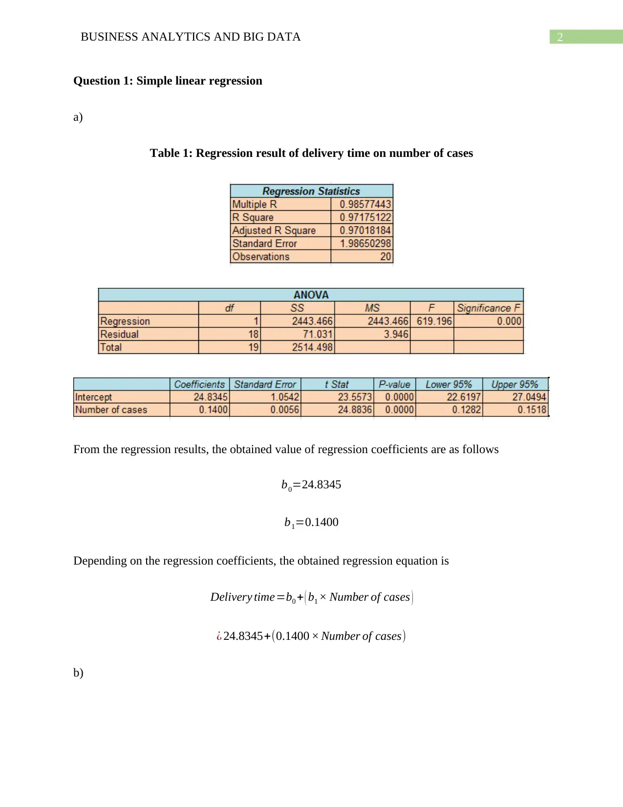
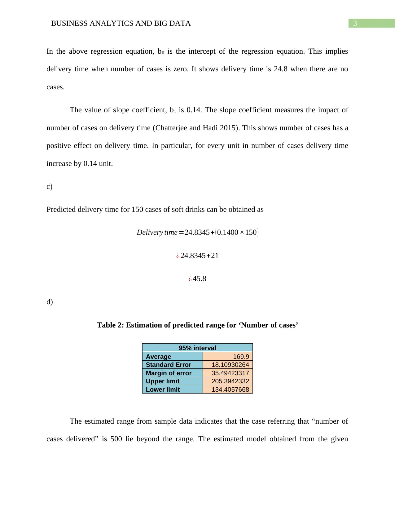
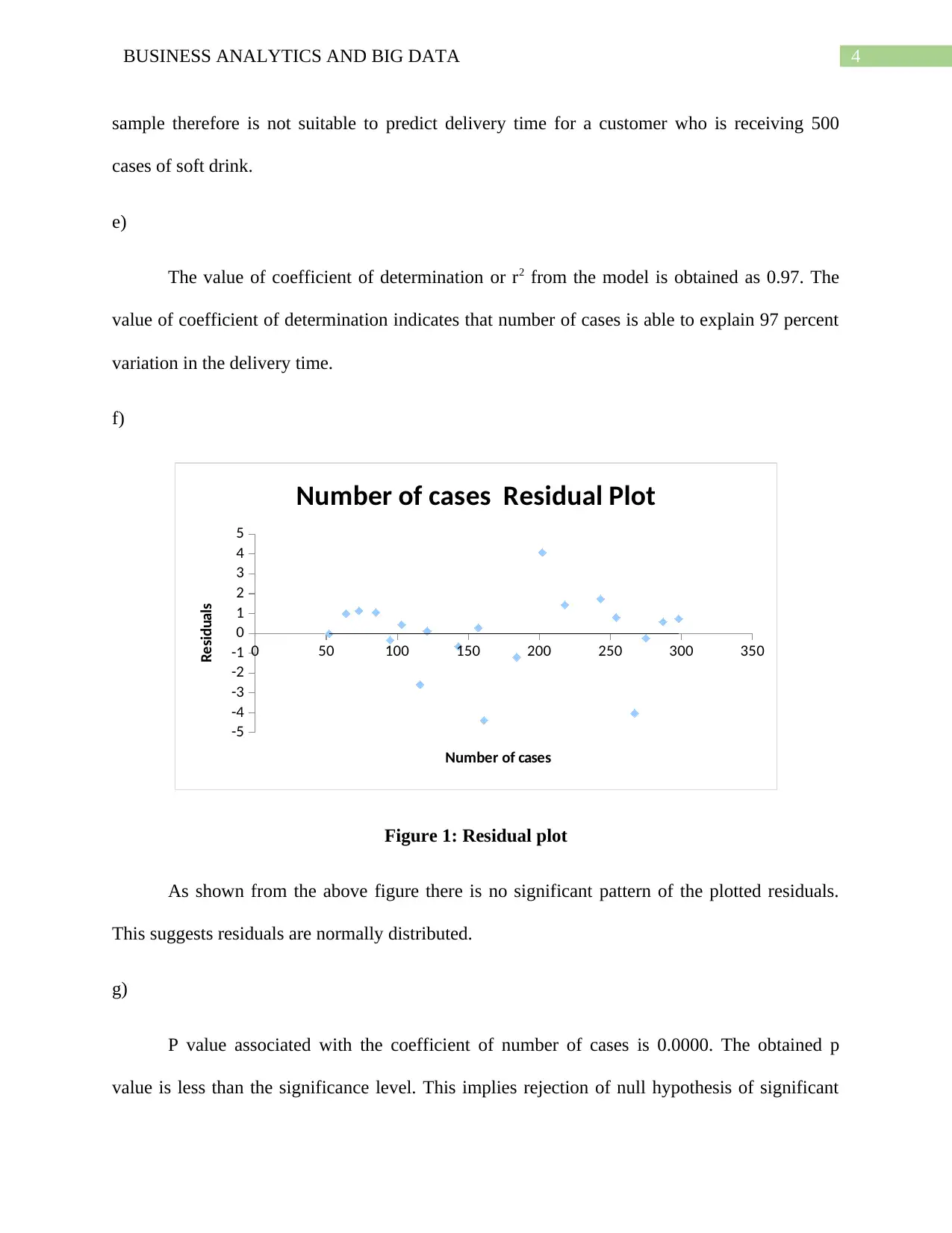
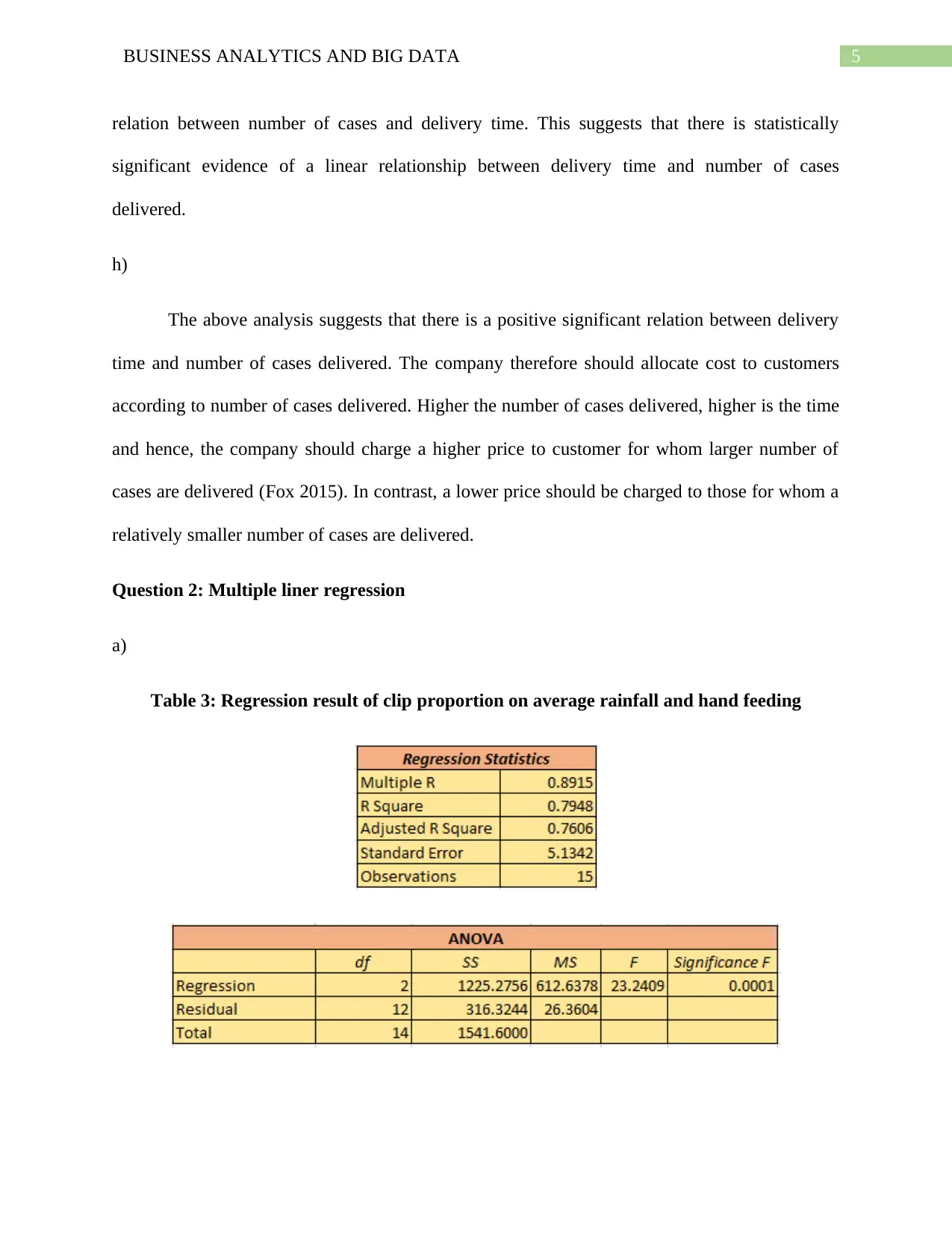
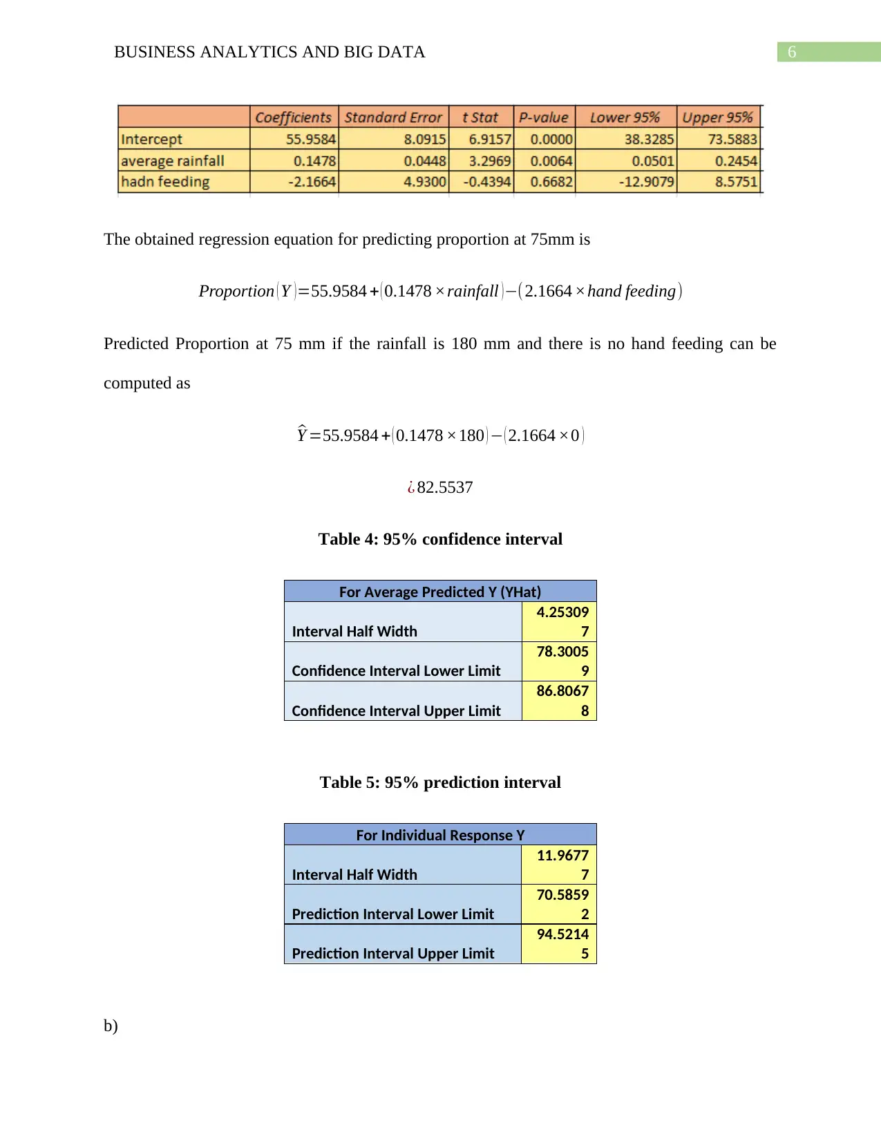
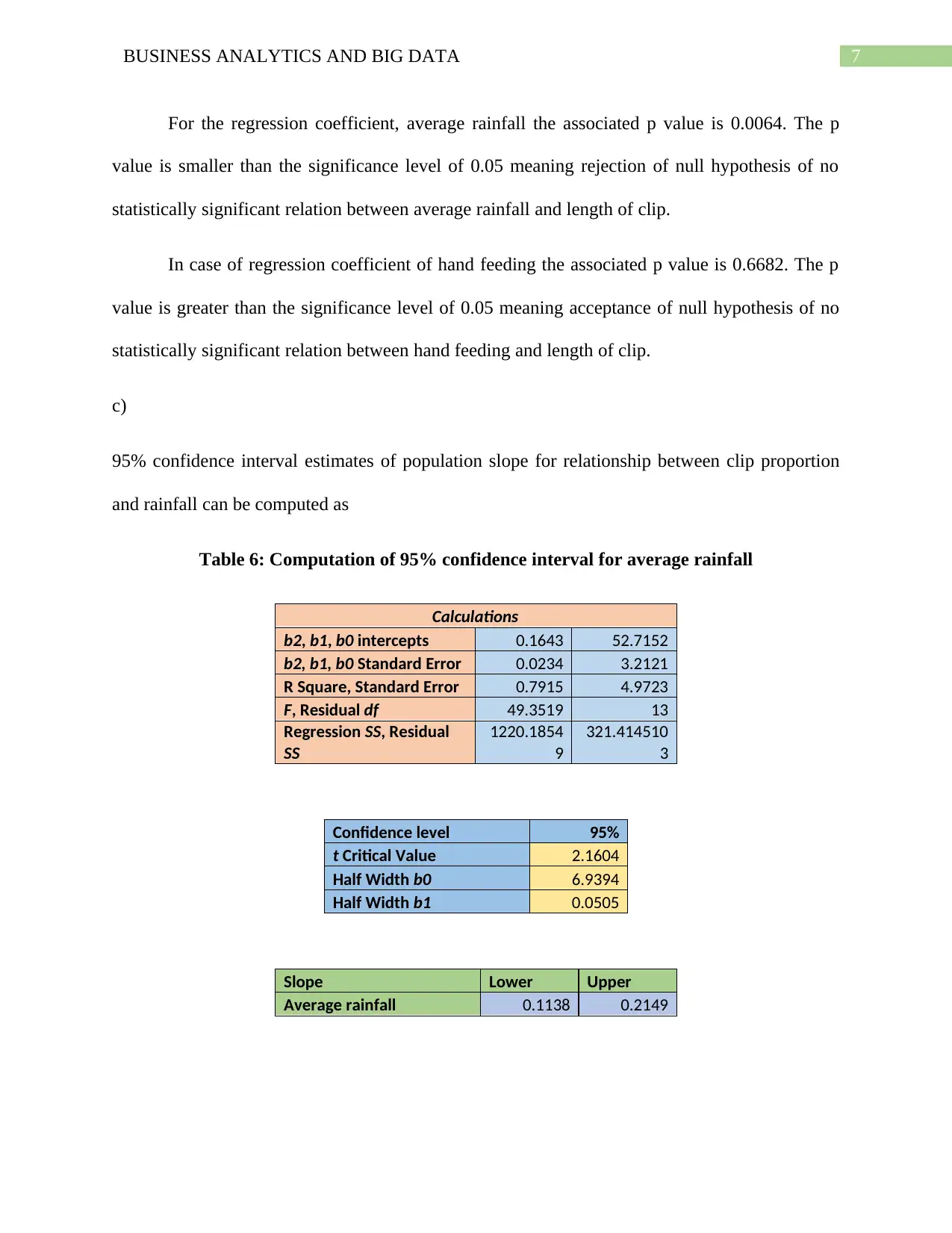
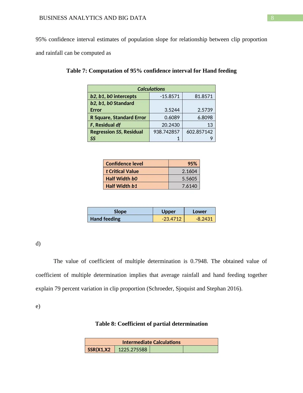
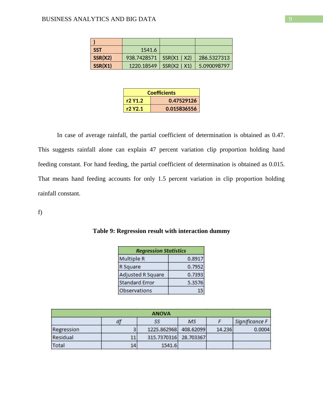
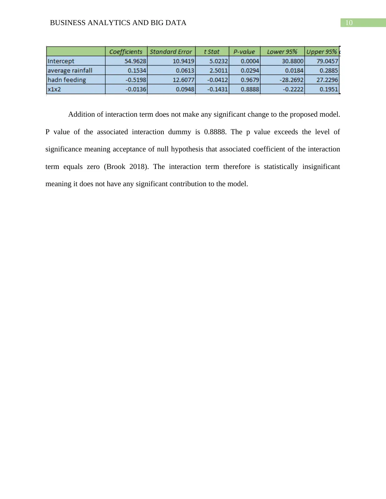
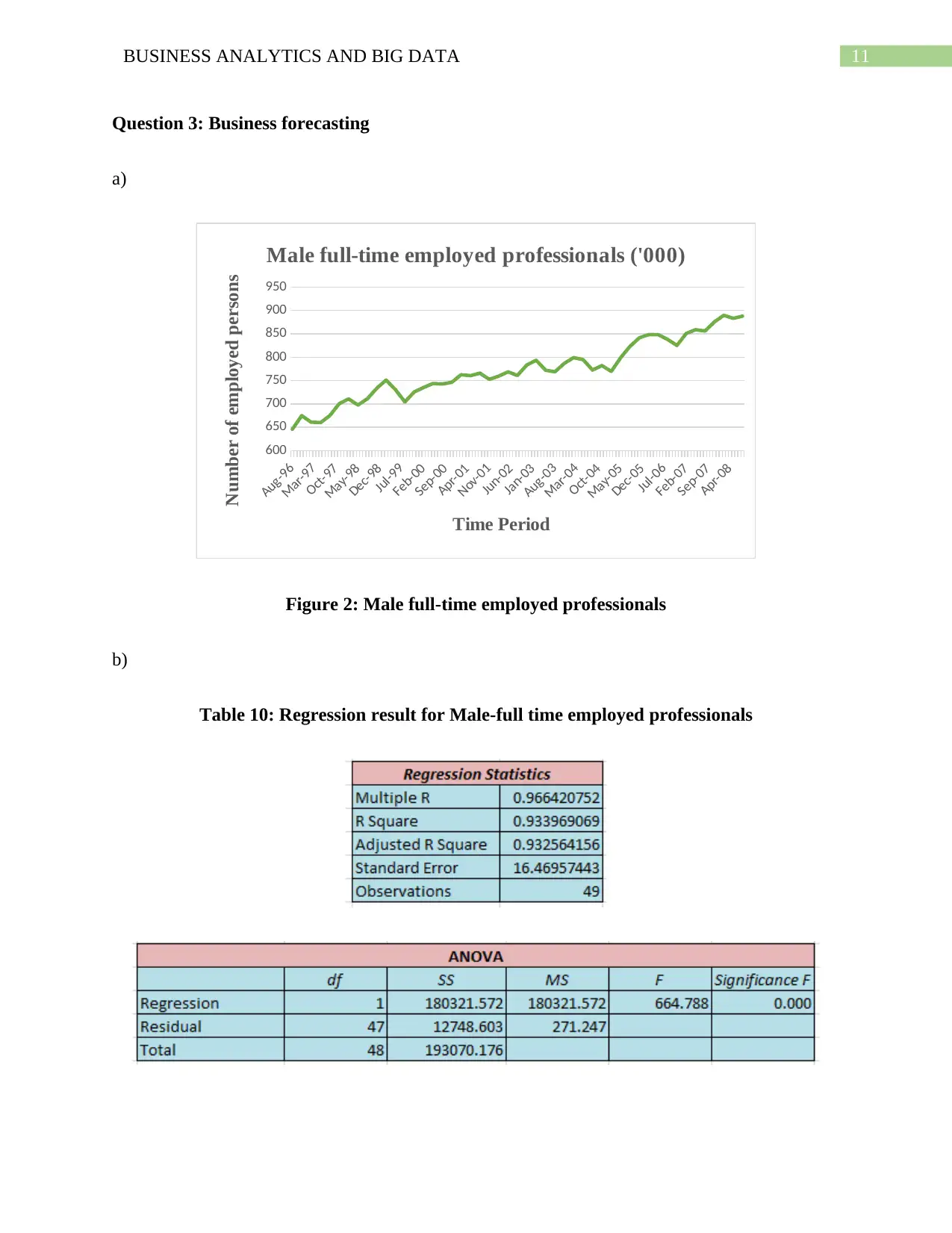
This document presents a comprehensive solution to a Business Analytics and Big Data assignment, focusing on regression analysis and business forecasting. The assignment includes three main questions. The first question explores simple linear regression, calculating regression coefficie...Read More

Running head: BUSINESS ANALYTICS AND BIG DATA
Business Analytics and Big Data
Name of the Student
Name of the University
Course ID

1BUSINESS ANALYTICS AND BIG DATA
Table of Contents
Question 1: Simple linear regression...............................................................................................2
Question 2: Multiple liner regression..............................................................................................5
Question 3: Business forecasting...................................................................................................10
References......................................................................................................................................14

2BUSINESS ANALYTICS AND BIG DATA
Question 1: Simple linear regression
a)
Table 1: Regression result of delivery time on number of cases
From the regression results, the obtained value of regression coefficients are as follows
b0=24.8345
b1=0.1400
Depending on the regression coefficients, the obtained regression equation is
Delivery time=b0 + ( b1 × Number of cases )
¿ 24.8345+(0.1400 × Number of cases)
b)

3BUSINESS ANALYTICS AND BIG DATA
In the above regression equation, b0 is the intercept of the regression equation. This implies
delivery time when number of cases is zero. It shows delivery time is 24.8 when there are no
cases.
The value of slope coefficient, b1 is 0.14. The slope coefficient measures the impact of
number of cases on delivery time (Chatterjee and Hadi 2015). This shows number of cases has a
positive effect on delivery time. In particular, for every unit in number of cases delivery time
increase by 0.14 unit.
c)
Predicted delivery time for 150 cases of soft drinks can be obtained as
Delivery time=24.8345+ ( 0.1400 ×150 )
¿ 24.8345+21
¿ 45.8
d)
Table 2: Estimation of predicted range for ‘Number of cases’
95% interval
Average 169.9
Standard Error 18.10930264
Margin of error 35.49423317
Upper limit 205.3942332
Lower limit 134.4057668
The estimated range from sample data indicates that the case referring that “number of
cases delivered” is 500 lie beyond the range. The estimated model obtained from the given

4BUSINESS ANALYTICS AND BIG DATA
sample therefore is not suitable to predict delivery time for a customer who is receiving 500
cases of soft drink.
e)
The value of coefficient of determination or r2 from the model is obtained as 0.97. The
value of coefficient of determination indicates that number of cases is able to explain 97 percent
variation in the delivery time.
f)
0 50 100 150 200 250 300 350
-5
-4
-3
-2
-1
0
1
2
3
4
5
Number of cases Residual Plot
Number of cases
Residuals
Figure 1: Residual plot
As shown from the above figure there is no significant pattern of the plotted residuals.
This suggests residuals are normally distributed.
g)
P value associated with the coefficient of number of cases is 0.0000. The obtained p
value is less than the significance level. This implies rejection of null hypothesis of significant

5BUSINESS ANALYTICS AND BIG DATA
relation between number of cases and delivery time. This suggests that there is statistically
significant evidence of a linear relationship between delivery time and number of cases
delivered.
h)
The above analysis suggests that there is a positive significant relation between delivery
time and number of cases delivered. The company therefore should allocate cost to customers
according to number of cases delivered. Higher the number of cases delivered, higher is the time
and hence, the company should charge a higher price to customer for whom larger number of
cases are delivered (Fox 2015). In contrast, a lower price should be charged to those for whom a
relatively smaller number of cases are delivered.
Question 2: Multiple liner regression
a)
Table 3: Regression result of clip proportion on average rainfall and hand feeding

6BUSINESS ANALYTICS AND BIG DATA
The obtained regression equation for predicting proportion at 75mm is
Proportion ( Y )=55.9584 + ( 0.1478 ×rainfall )−(2.1664 ×hand feeding)
Predicted Proportion at 75 mm if the rainfall is 180 mm and there is no hand feeding can be
computed as
^Y =55.9584 + ( 0.1478 ×180 ) − ( 2.1664 ×0 )
¿ 82.5537
Table 4: 95% confidence interval
For Average Predicted Y (YHat)
Interval Half Width
4.25309
7
Confidence Interval Lower Limit
78.3005
9
Confidence Interval Upper Limit
86.8067
8
Table 5: 95% prediction interval
For Individual Response Y
Interval Half Width
11.9677
7
Prediction Interval Lower Limit
70.5859
2
Prediction Interval Upper Limit
94.5214
5
b)

7BUSINESS ANALYTICS AND BIG DATA
For the regression coefficient, average rainfall the associated p value is 0.0064. The p
value is smaller than the significance level of 0.05 meaning rejection of null hypothesis of no
statistically significant relation between average rainfall and length of clip.
In case of regression coefficient of hand feeding the associated p value is 0.6682. The p
value is greater than the significance level of 0.05 meaning acceptance of null hypothesis of no
statistically significant relation between hand feeding and length of clip.
c)
95% confidence interval estimates of population slope for relationship between clip proportion
and rainfall can be computed as
Table 6: Computation of 95% confidence interval for average rainfall
Calculations
b2, b1, b0 intercepts 0.1643 52.7152
b2, b1, b0 Standard Error 0.0234 3.2121
R Square, Standard Error 0.7915 4.9723
F, Residual df 49.3519 13
Regression SS, Residual
SS
1220.1854
9
321.414510
3
Confidence level 95%
t Critical Value 2.1604
Half Width b0 6.9394
Half Width b1 0.0505
Slope Lower Upper
Average rainfall 0.1138 0.2149

8BUSINESS ANALYTICS AND BIG DATA
95% confidence interval estimates of population slope for relationship between clip proportion
and rainfall can be computed as
Table 7: Computation of 95% confidence interval for Hand feeding
Calculations
b2, b1, b0 intercepts -15.8571 81.8571
b2, b1, b0 Standard
Error 3.5244 2.5739
R Square, Standard Error 0.6089 6.8098
F, Residual df 20.2430 13
Regression SS, Residual
SS
938.742857
1
602.857142
9
Confidence level 95%
t Critical Value 2.1604
Half Width b0 5.5605
Half Width b1 7.6140
Slope Upper Lower
Hand feeding -23.4712 -8.2431
d)
The value of coefficient of multiple determination is 0.7948. The obtained value of
coefficient of multiple determination implies that average rainfall and hand feeding together
explain 79 percent variation in clip proportion (Schroeder, Sjoquist and Stephan 2016).
e)
Table 8: Coefficient of partial determination
Intermediate Calculations
SSR(X1,X2 1225.275588

9BUSINESS ANALYTICS AND BIG DATA
)
SST 1541.6
SSR(X2) 938.7428571 SSR(X1 | X2) 286.5327313
SSR(X1) 1220.18549 SSR(X2 | X1) 5.090098797
Coefficients
r2 Y1.2 0.47529126
r2 Y2.1 0.015836556
In case of average rainfall, the partial coefficient of determination is obtained as 0.47.
This suggests rainfall alone can explain 47 percent variation clip proportion holding hand
feeding constant. For hand feeding, the partial coefficient of determination is obtained as 0.015.
That means hand feeding accounts for only 1.5 percent variation in clip proportion holding
rainfall constant.
f)
Table 9: Regression result with interaction dummy

10BUSINESS ANALYTICS AND BIG DATA
Addition of interaction term does not make any significant change to the proposed model.
P value of the associated interaction dummy is 0.8888. The p value exceeds the level of
significance meaning acceptance of null hypothesis that associated coefficient of the interaction
term equals zero (Brook 2018). The interaction term therefore is statistically insignificant
meaning it does not have any significant contribution to the model.

11BUSINESS ANALYTICS AND BIG DATA
Question 3: Business forecasting
a)
Aug-96
Mar-97
Oct-97
May-98
Dec-98
Jul-99
Feb-00
Sep-00
Apr-01
Nov-01
Jun-02
Jan-03
Aug-03
Mar-04
Oct-04
May-05
Dec-05
Jul-06
Feb-07
Sep-07
Apr-08
600
650
700
750
800
850
900
950
Male full-time employed professionals ('000)
Time Period
Number of employed persons
Figure 2: Male full-time employed professionals
b)
Table 10: Regression result for Male-full time employed professionals

12BUSINESS ANALYTICS AND BIG DATA
The estimate liner trend equation is obtained as
Employment=669.0076+(4.2895× time)
0 10 20 30 40 50 60
600
650
700
750
800
850
900
950
f(x) = 4.28954081632653 x + 669.077551020408
R² = 0.933969068965788
Male full-time employed professionals ('000)
Time-period
Number of employed
professionals
Figure 3: Trend line for full time employment
c)
Using the linear trend equation, the forecasted value of full-time employment in November
quarter 2008 and February quarter 2009 can be obtained as
Employment2008=669.0076+ ( 4.2895 × 49 )
¿ 879.3

13BUSINESS ANALYTICS AND BIG DATA
Employment2009=669.0076+ ( 4.2895 ×50 )
¿ 883.6
Table 11: Number of employed professionals in Nov-2008 and Feb-2009
Forecast
Year Employment
Nov_20
08 879.3
Feb_200
9 883.6
d)
Given the data set, it is reasonable to forecast employment in this way. The linear trend
fitted for predicting full-time employed professionals. The obtained value of correlation
coefficient associated with the linear trend is 0.934. Value of correlation coefficient closer to 1
implies a strong degree of association. The obtained model has overall statistical significance
(Chatterjee and Hadi 2015). Also the deviation between observed number of male full-time
employed professionals and that of predicted male full time employed professionals is very small
indicating that the model gives a good prediction and therefore can be used to predict
employment for future quarters.

14BUSINESS ANALYTICS AND BIG DATA
0 10 20 30 40 50 60
0
200
400
600
800
1000
Time Line Fit Plot
Male full-time employed professionals ('000) Predicted Male full-time employed professionals ('000)
Time
Male full-time employed professionals
('000)
Figure 4: Fitted value and observed value

15BUSINESS ANALYTICS AND BIG DATA
References
Brook, R.J., 2018. Applied regression analysis and experimental design. Routledge.
Chatterjee, S. and Hadi, A.S., 2015. Regression analysis by example. John Wiley & Sons.
Fox, J., 2015. Applied regression analysis and generalized linear models. Sage Publications.
Schroeder, L.D., Sjoquist, D.L. and Stephan, P.E., 2016. Understanding regression analysis: An
introductory guide (Vol. 57). Sage Publications.